FISH 6003: Week 7, GLMs Part 2

6003 Week 7, GLMs 2

Transcript

1. Chapter 7: Generalized linear models, Part 2 CatchRate ~ Poisson (μ ij ) E(CatchRate) = μ ij Log(μ ij ) = GearType ij + Temperature ij + FleetDeployment i FleetDeployment i ~ N(0, σ2) Using lme4: m <- glmer(CatchRate ~ GearType + Temperature + (1 | FleetDeployment), family = poisson) FISH 6003 FISH 6003: Statistics and Study Design for Fisheries Brett Favaro 2017 This work is licensed under a Creative Commons Attribution 4.0 International License
2. Land Acknowledgment We would like to respectfully acknowledge the territory in which we gather as the ancestral homelands of the Beothuk, and the island of Newfoundland as the ancestral homelands of the Mi’kmaq and Beothuk. We would also like to recognize the Inuit of Nunatsiavut and NunatuKavut and the Innu of Nitassinan, and their ancestors, as the original people of Labrador. We strive for respectful partnerships with all the peoples of this province as we search for collective healing and true reconciliation and honour this beautiful land together. http://www.mun.ca/aboriginal_affairs/
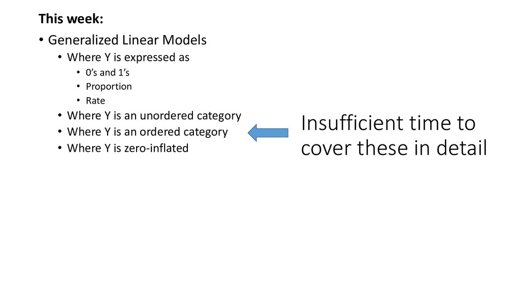
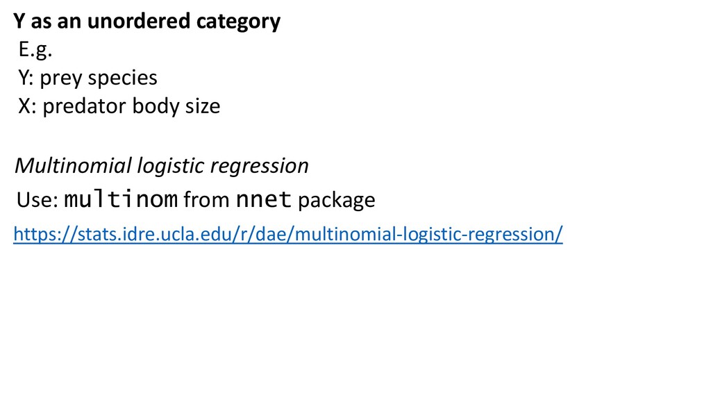
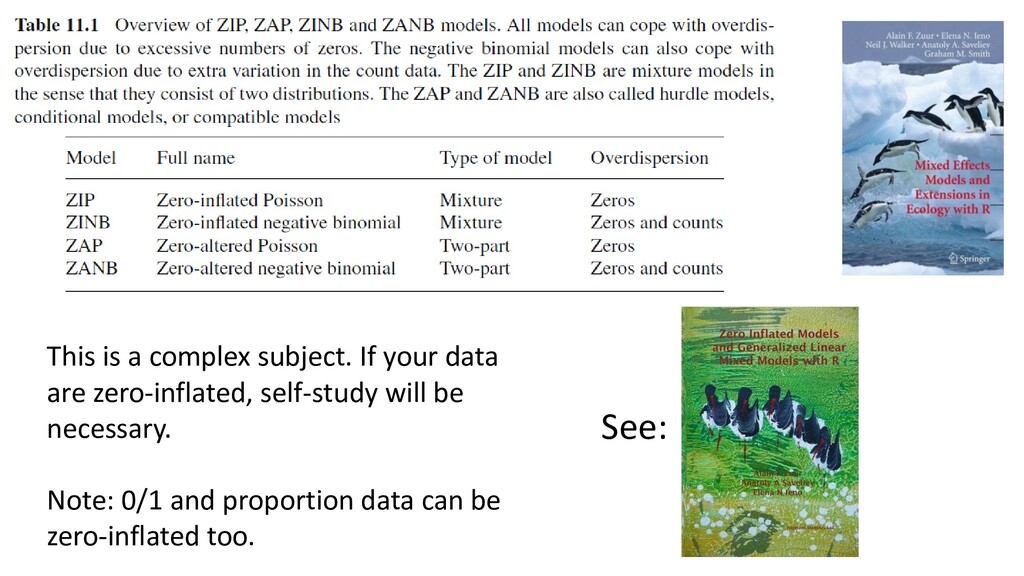
3. This week: • Generalized Linear Models • Where Y is expressed as • 0’s and 1’s • Proportion • Rate • Where Y is an unordered category • Where Y is an ordered category • Where Y is zero-inflated Insufficient time to cover these in detail
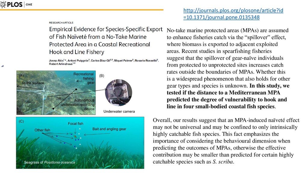
4. http://journals.plos.org/plosone/article?id =10.1371/journal.pone.0135348 No-take marine protected areas (MPAs) are assumed to enhance fisheries catch via the “spillover” effect, where biomass is exported to adjacent exploited areas. Recent studies in spearfishing fisheries suggest that the spillover of gear-naïve individuals from protected to unprotected sites increases catch rates outside the boundaries of MPAs. Whether this is a widespread phenomenon that also holds for other gear types and species is unknown. In this study, we tested if the distance to a Mediterranean MPA predicted the degree of vulnerability to hook and line in four small-bodied coastal fish species. Overall, our results suggest that an MPA-induced naïveté effect may not be universal and may be confined to only intrinsically highly catchable fish species. This fact emphasizes the importance of considering the behavioural dimension when predicting the outcomes of MPAs, otherwise the effective contribution may be smaller than predicted for certain highly catchable species such as S. scriba.
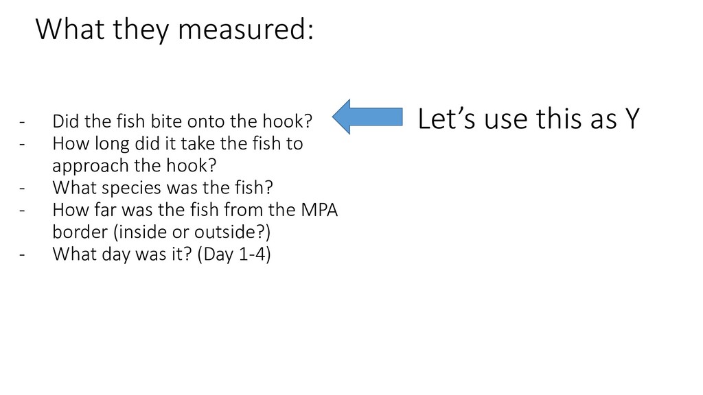
5. What they measured: - Did the fish bite onto the hook? - How long did it take the fish to approach the hook? - What species was the fish? - How far was the fish from the MPA border (inside or outside?) - What day was it? (Day 1-4) Let’s use this as Y
6. Distribution of response Predictor function ηi = β0 + β1 Lt_Si + β2 Distance_mi + Speciesi Link (eta) logit(πi ) = ηi Still need: • Independence • Fixed X Don’t need: • Normality • No overdispersion Hard to assess: • No patterns in residuals indicating lack of fit Event: Yes/no. 1/0 Eventi ~ B(πi, 1) E(Yi ) = πi Var(Yi ) = πi * (1 - πi )
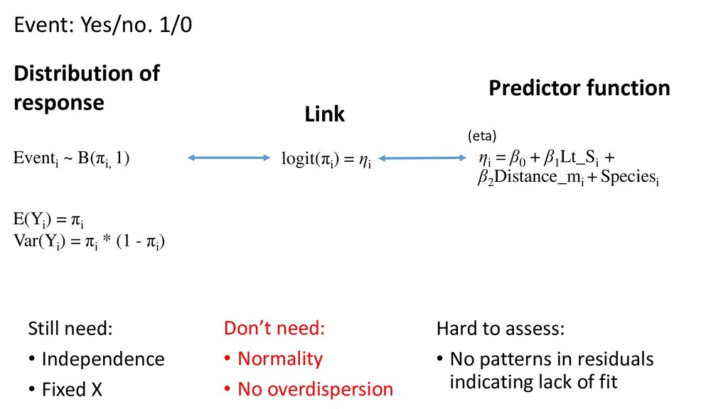
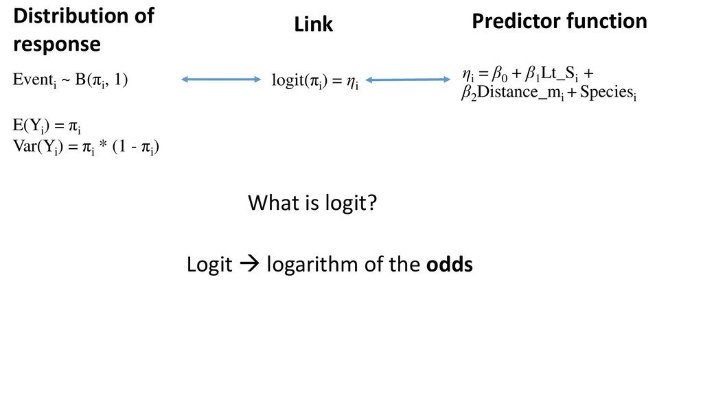
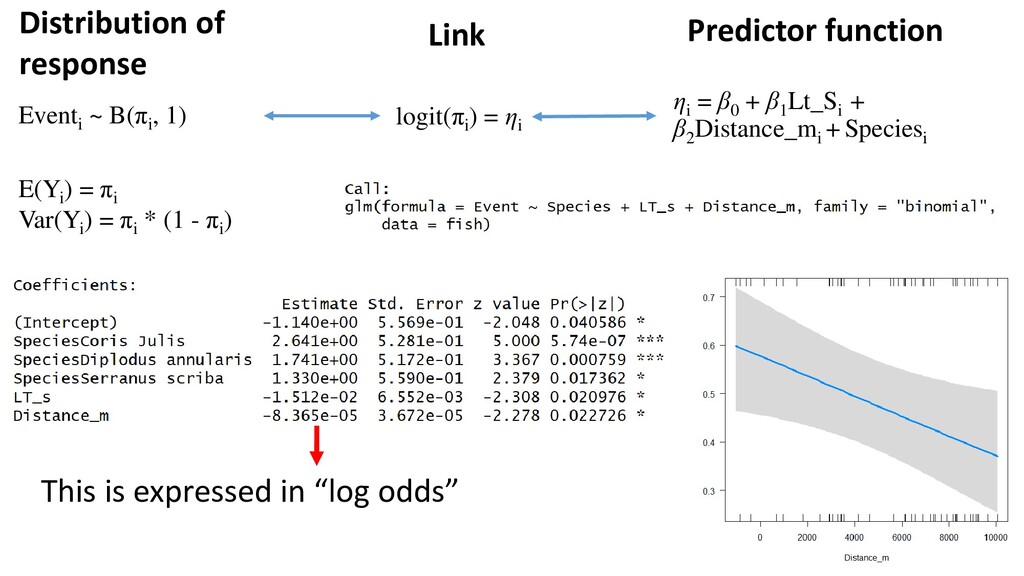
7. logit(πi ) = ηi Eventi ~ B(πi , 1) E(Yi ) = πi Var(Yi ) = πi * (1 - πi ) Distribution of response Predictor function Link Logit → logarithm of the odds What is logit? ηi = β0 + β1 Lt_Si + β2 Distance_mi + Speciesi
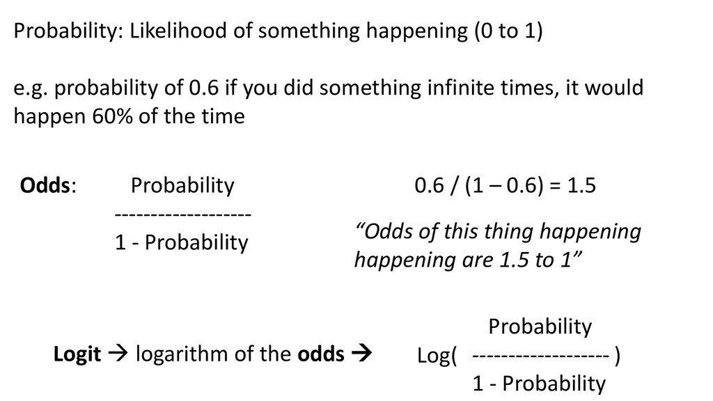
8. Odds: Probability ------------------- 1 - Probability Probability: Likelihood of something happening (0 to 1) e.g. probability of 0.6 if you did something infinite times, it would happen 60% of the time 0.6 / (1 – 0.6) = 1.5 “Odds of this thing happening happening are 1.5 to 1” Logit → logarithm of the odds → Probability ------------------- 1 - Probability Log( )
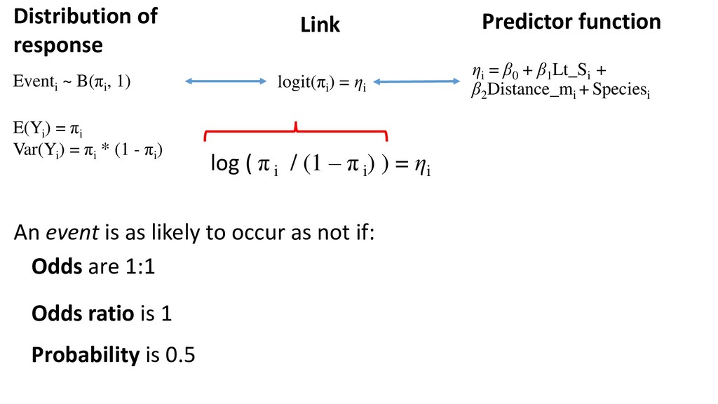
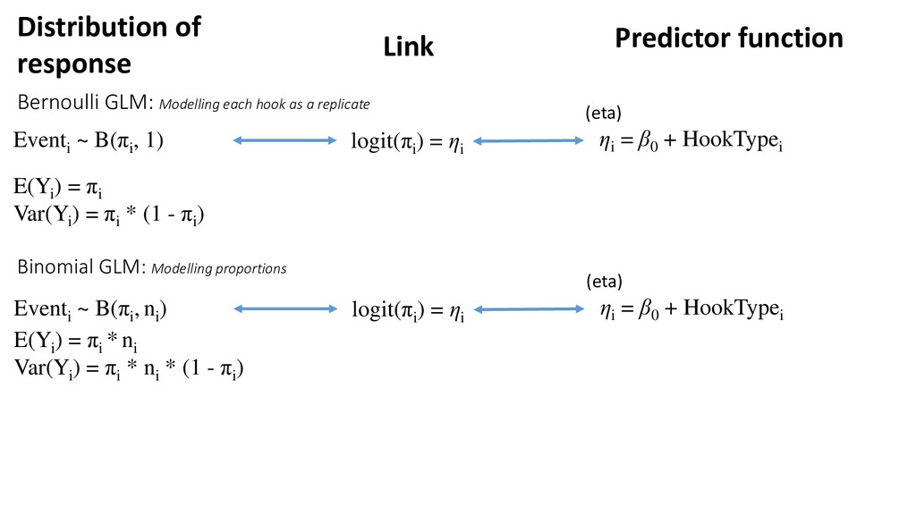
9. logit(πi ) = ηi Eventi ~ B(πi , 1) E(Yi ) = πi Var(Yi ) = πi * (1 - πi ) Distribution of response Predictor function Link log ( π i / (1 – π i ) ) = ηi Odds are 1:1 Probability is 0.5 Odds ratio is 1 An event is as likely to occur as not if: ηi = β0 + β1 Lt_Si + β2 Distance_mi + Speciesi
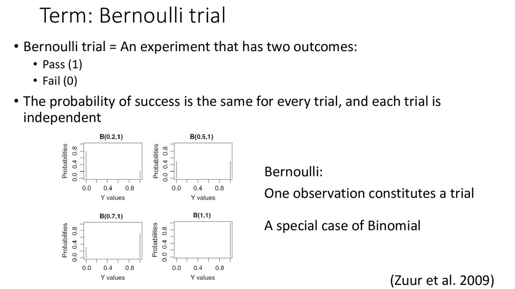
10. Term: Bernoulli trial • Bernoulli trial = An experiment that has two outcomes: • Pass (1) • Fail (0) • The probability of success is the same for every trial, and each trial is independent (Zuur et al. 2009) Bernoulli: One observation constitutes a trial A special case of Binomial
11. logit(πi ) = ηi Eventi ~ B(πi , 1) E(Yi ) = πi Var(Yi ) = πi * (1 - πi ) Distribution of response Predictor function Link This is expressed in “log odds” ηi = β0 + β1 Lt_Si + β2 Distance_mi + Speciesi
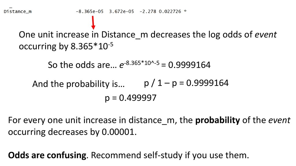
12. One unit increase in Distance_m decreases the log odds of event occurring by 8.365*10-5 So the odds are… e-8.365*10^-5 = 0.9999164 For every one unit increase in distance_m, the probability of the event occurring decreases by 0.00001. Odds are confusing. Recommend self-study if you use them. And the probability is… p / 1 – p = 0.9999164 p = 0.499997
13. P(Event) P(Event) P(Event)
14. Do Exercise 1
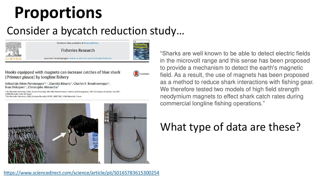
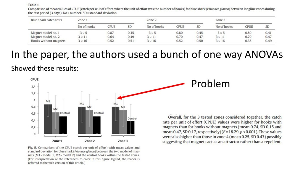
15. Proportions What type of data are these? Consider a bycatch reduction study… https://www.sciencedirect.com/science/article/pii/S0165783615300254 “Sharks are well known to be able to detect electric fields in the microvolt range and this sense has been proposed to provide a mechanism to detect the earth's magnetic field. As a result, the use of magnets has been proposed as a method to reduce shark interactions with fishing gear. We therefore tested two models of high field strength neodymium magnets to effect shark catch rates during commercial longline fishing operations.”
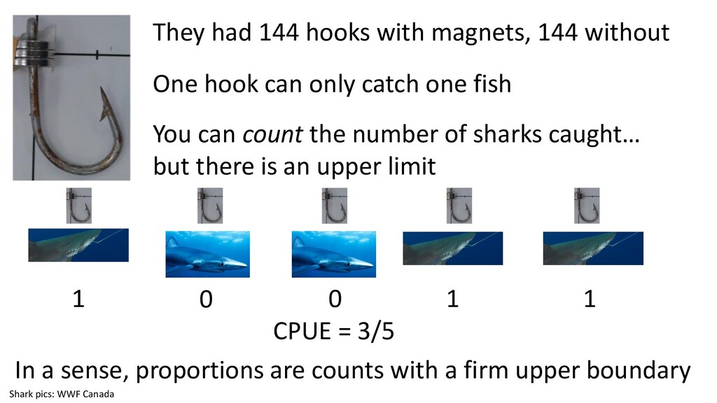
16. In a sense, proportions are counts with a firm upper boundary One hook can only catch one fish They had 144 hooks with magnets, 144 without You can count the number of sharks caught… but there is an upper limit Shark pics: WWF Canada 1 0 0 1 1 CPUE = 3/5 1
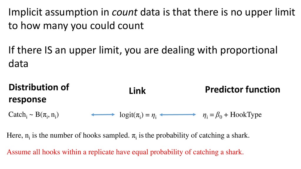
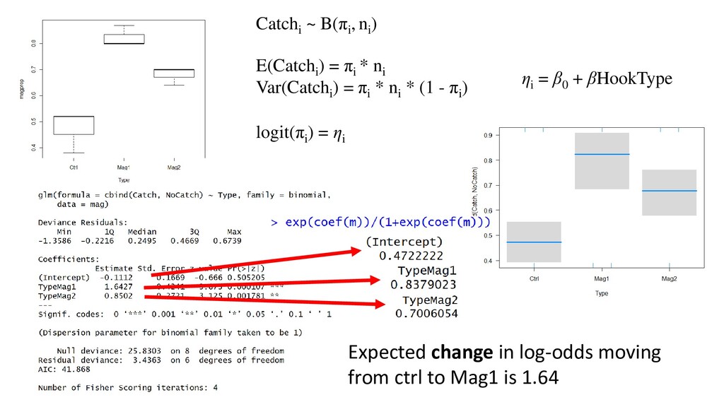
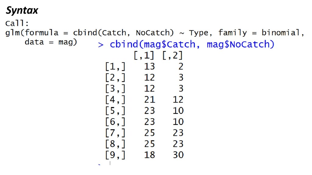
17. Implicit assumption in count data is that there is no upper limit to how many you could count If there IS an upper limit, you are dealing with proportional data ηi = β0 + HookType logit(πi ) = ηi Catchi ~ B(πi , ni ) Distribution of response Predictor function Link Here, ni is the number of hooks sampled. πi is the probability of catching a shark. Assume all hooks within a replicate have equal probability of catching a shark.
18. 1 1 1 1 1 1 1 0 0 0 0 0 0 1 0 3/5 Yi 4/5 1/5 Replicate 1 2 3
19. In the paper, the authors used a bunch of one way ANOVAs Showed these results: Problem
20. Catchi ~ B(πi , ni ) logit(πi ) = ηi E(Catchi ) = πi * ni Var(Catchi ) = πi * ni * (1 - πi ) ηi = β0 + βHookType Expected change in log-odds moving from ctrl to Mag1 is 1.64
21. Syntax
22. Beware tiny sample size:
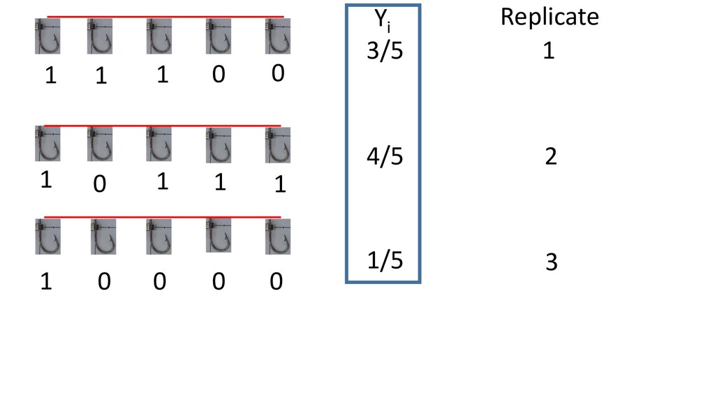
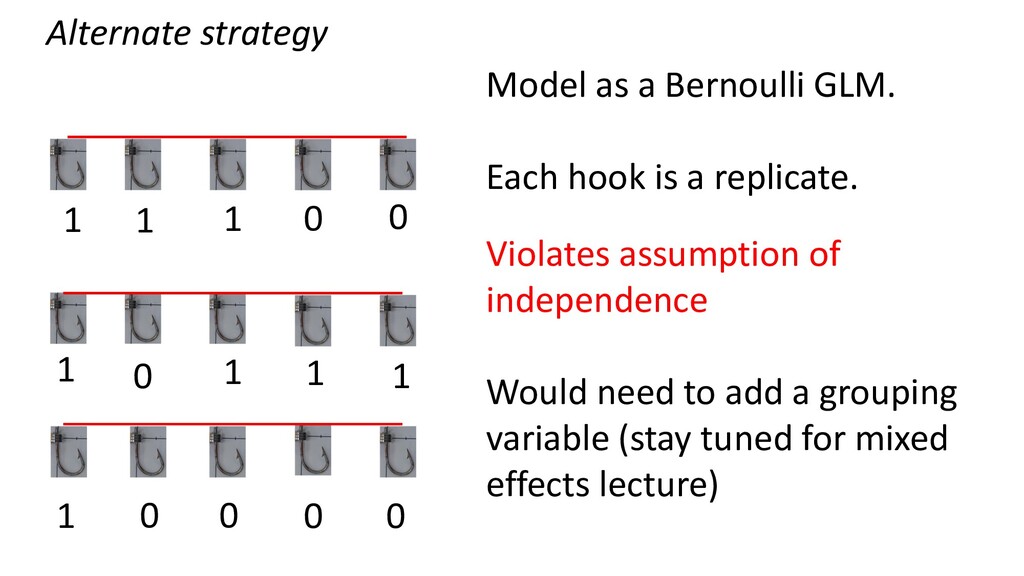
23. 1 1 1 1 1 1 1 0 0 0 0 0 0 1 0 Model as a Bernoulli GLM. Each hook is a replicate. Violates assumption of independence Would need to add a grouping variable (stay tuned for mixed effects lecture) Alternate strategy
24. Bernoulli GLM: Modelling each hook as a replicate Distribution of response Predictor function ηi = β0 + HookTypei Link (eta) logit(πi ) = ηi Eventi ~ B(πi , 1) E(Yi ) = πi Var(Yi ) = πi * (1 - πi ) ηi = β0 + HookTypei (eta) logit(πi ) = ηi Eventi ~ B(πi , ni ) E(Yi ) = πi * ni Var(Yi ) = πi * ni * (1 - πi ) Binomial GLM: Modelling proportions
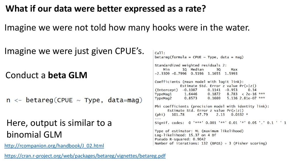
25. What if our data were better expressed as a rate? Imagine we were not told how many hooks were in the water. Imagine we were just given CPUE’s. Conduct a beta GLM https://cran.r-project.org/web/packages/betareg/vignettes/betareg.pdf Here, output is similar to a binomial GLM http://rcompanion.org/handbook/J_02.html
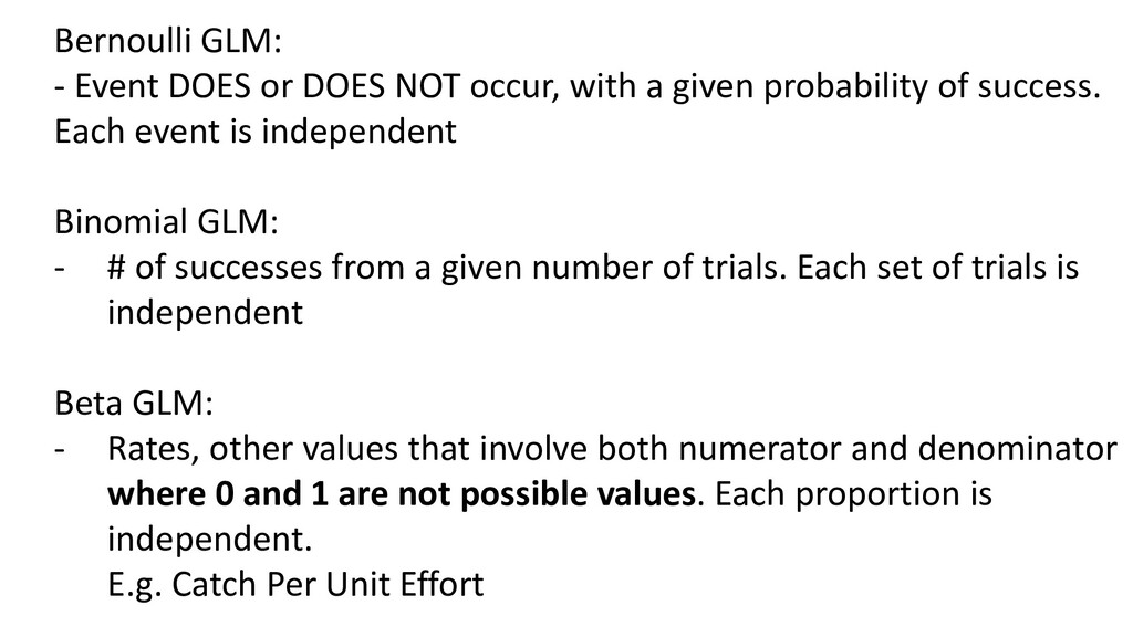
26. Bernoulli GLM: - Event DOES or DOES NOT occur, with a given probability of success. Each event is independent Binomial GLM: - # of successes from a given number of trials. Each set of trials is independent Beta GLM: - Rates, other values that involve both numerator and denominator where 0 and 1 are not possible values. Each proportion is independent. E.g. Catch Per Unit Effort
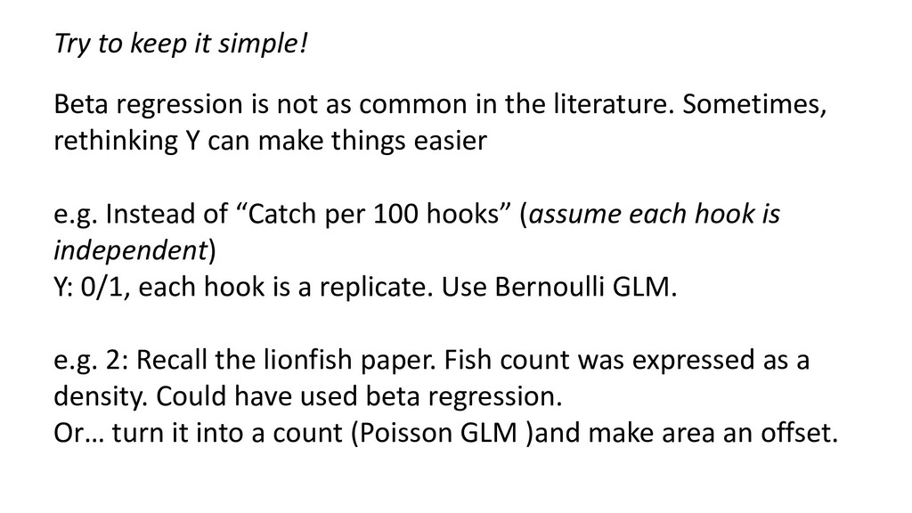
27. Try to keep it simple! Beta regression is not as common in the literature. Sometimes, rethinking Y can make things easier e.g. Instead of “Catch per 100 hooks” (assume each hook is independent) Y: 0/1, each hook is a replicate. Use Bernoulli GLM. e.g. 2: Recall the lionfish paper. Fish count was expressed as a density. Could have used beta regression. Or… turn it into a count (Poisson GLM )and make area an offset.
28. Do Exercise 2
29. Y as an unordered category https://stats.idre.ucla.edu/r/dae/multinomial-logistic-regression/ E.g. Y: prey species X: predator body size Use: multinom from nnet package Multinomial logistic regression
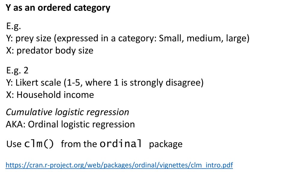
30. Y as an ordered category Cumulative logistic regression AKA: Ordinal logistic regression E.g. Y: prey size (expressed in a category: Small, medium, large) X: predator body size E.g. 2 Y: Likert scale (1-5, where 1 is strongly disagree) X: Household income Use clm() from the ordinal package https://cran.r-project.org/web/packages/ordinal/vignettes/clm_intro.pdf
31. Recap Y data Distribution Do it in… Continuous Gaussian lm() Count Poisson glm(family = Poisson) Count – overdispersed Negative-binomial glm.nb() 0’s and 1’s (single observations that did or did not occur) Bernoulli glm(family = binomial) Proportion Binomial glm(Y = cbind(Success, Failure), family = binomial) Rate Beta betareg() Unordered categories Multinomial multinom() Ordered categories Cumulative logistics regression clm()
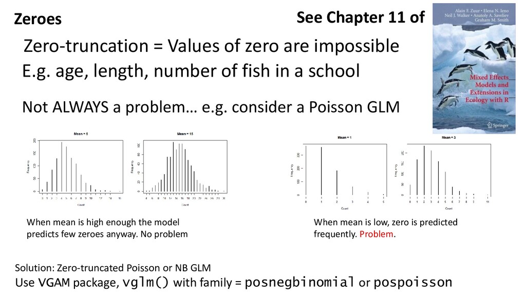
32. Zeroes Zero-truncation = Values of zero are impossible E.g. age, length, number of fish in a school Not ALWAYS a problem… e.g. consider a Poisson GLM When mean is high enough the model predicts few zeroes anyway. No problem When mean is low, zero is predicted frequently. Problem. See Chapter 11 of Solution: Zero-truncated Poisson or NB GLM Use VGAM package, vglm() with family = posnegbinomial or pospoisson
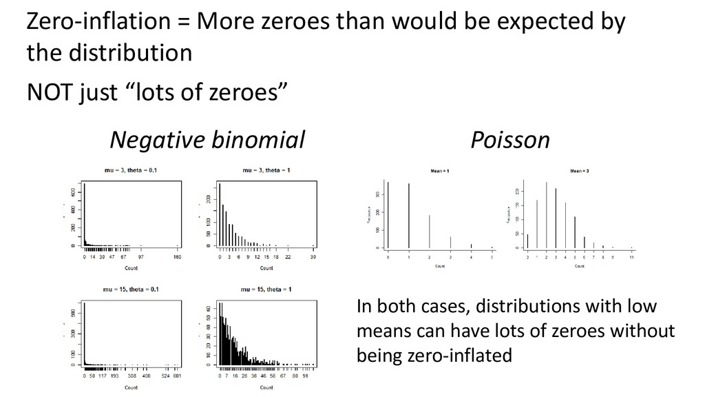
33. Zero-inflation = More zeroes than would be expected by the distribution NOT just “lots of zeroes” Poisson Negative binomial In both cases, distributions with low means can have lots of zeroes without being zero-inflated
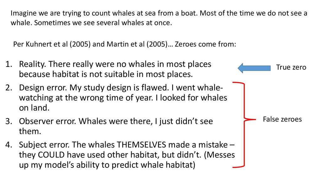
34. Per Kuhnert et al (2005) and Martin et al (2005)… Zeroes come from: 1. Reality. There really were no whales in most places because habitat is not suitable in most places. 2. Design error. My study design is flawed. I went whale- watching at the wrong time of year. I looked for whales on land. 3. Observer error. Whales were there, I just didn’t see them. 4. Subject error. The whales THEMSELVES made a mistake – they COULD have used other habitat, but didn’t. (Messes up my model’s ability to predict whale habitat) Imagine we are trying to count whales at sea from a boat. Most of the time we do not see a whale. Sometimes we see several whales at once. True zero False zeroes
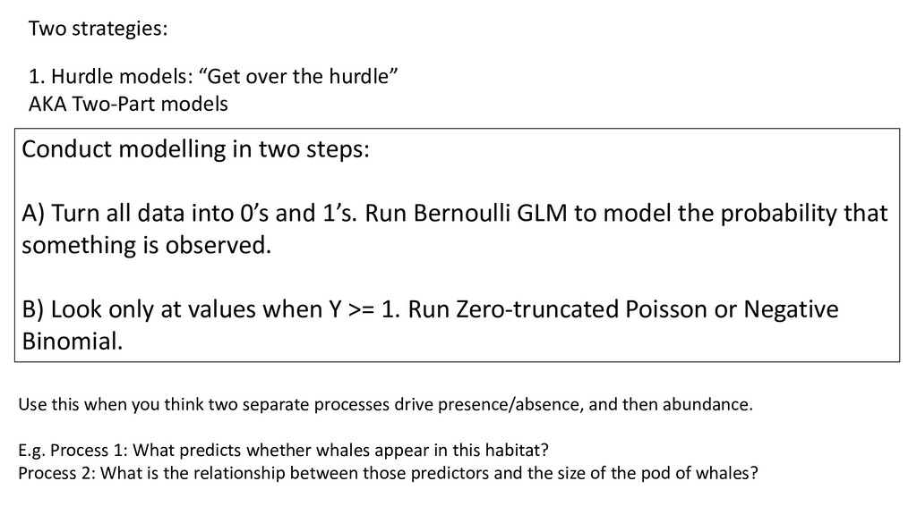
35. Two strategies: 1. Hurdle models: “Get over the hurdle” AKA Two-Part models Conduct modelling in two steps: A) Turn all data into 0’s and 1’s. Run Bernoulli GLM to model the probability that something is observed. B) Look only at values when Y >= 1. Run Zero-truncated Poisson or Negative Binomial. Use this when you think two separate processes drive presence/absence, and then abundance. E.g. Process 1: What predicts whether whales appear in this habitat? Process 2: What is the relationship between those predictors and the size of the pod of whales?
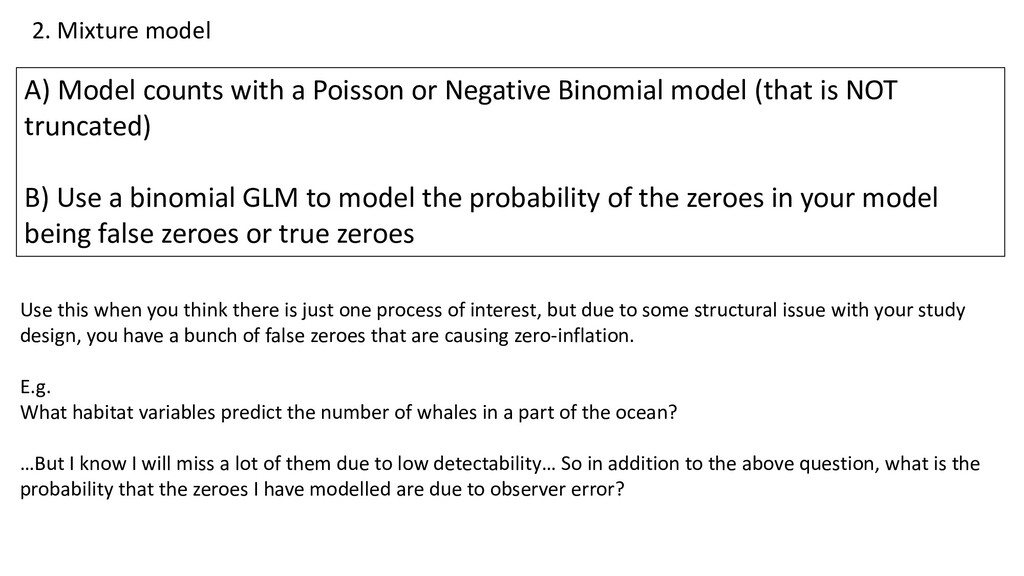
36. 2. Mixture model A) Model counts with a Poisson or Negative Binomial model (that is NOT truncated) B) Use a binomial GLM to model the probability of the zeroes in your model being false zeroes or true zeroes Use this when you think there is just one process of interest, but due to some structural issue with your study design, you have a bunch of false zeroes that are causing zero-inflation. E.g. What habitat variables predict the number of whales in a part of the ocean? …But I know I will miss a lot of them due to low detectability… So in addition to the above question, what is the probability that the zeroes I have modelled are due to observer error?
37. This is a complex subject. If your data are zero-inflated, self-study will be necessary. Note: 0/1 and proportion data can be zero-inflated too. See:
38. How do I test for zero-inflation? Zuur et al (2016) You may detect many zeroes during data exploration But it’s not always clear whether data are zero-inflated Use simulation to evaluate
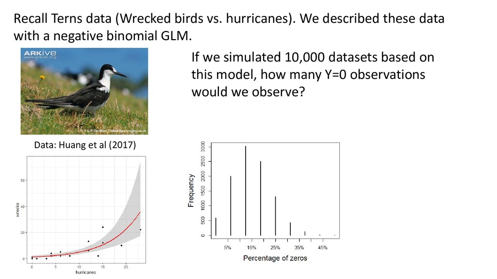
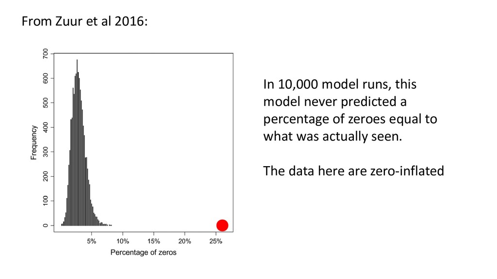
39. Data: Huang et al (2017) Recall Terns data (Wrecked birds vs. hurricanes). We described these data with a negative binomial GLM. If we simulated 10,000 datasets based on this model, how many Y=0 observations would we observe?
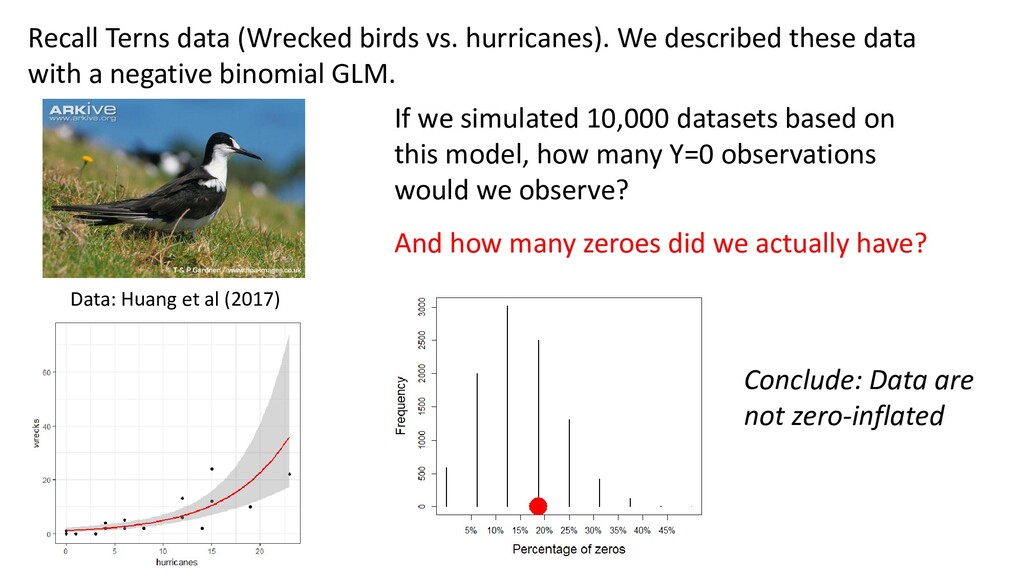
40. Data: Huang et al (2017) Recall Terns data (Wrecked birds vs. hurricanes). We described these data with a negative binomial GLM. If we simulated 10,000 datasets based on this model, how many Y=0 observations would we observe? And how many zeroes did we actually have? Conclude: Data are not zero-inflated
41. If we simulated 10,000 datasets based on this model, how many Y=0 observations would we observe? Recall: Shark magnets. Binomial GLM. Y: Probability of catching a shark.
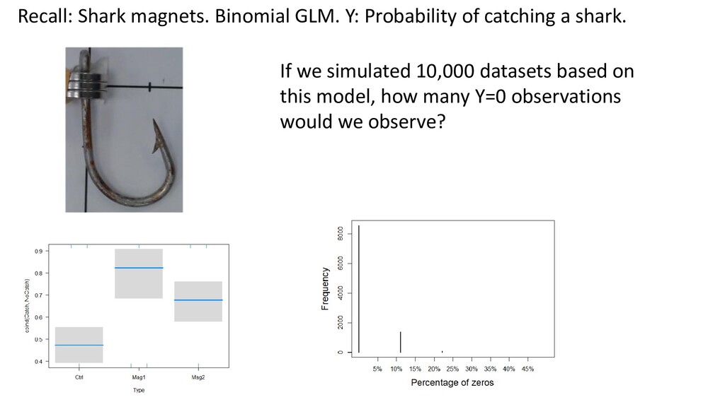
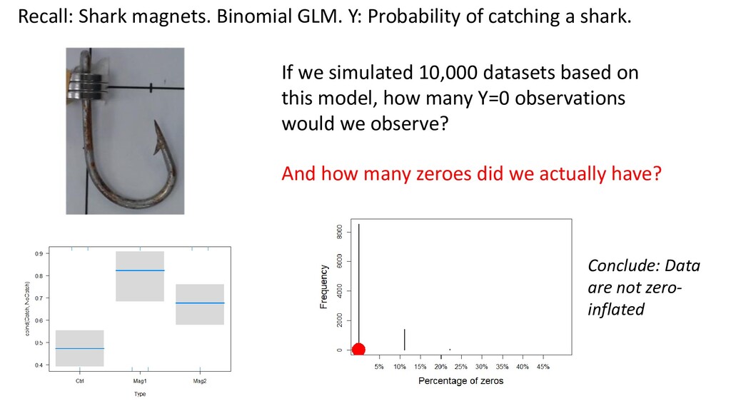
42. If we simulated 10,000 datasets based on this model, how many Y=0 observations would we observe? Recall: Shark magnets. Binomial GLM. Y: Probability of catching a shark. And how many zeroes did we actually have? Conclude: Data are not zero- inflated
43. From Zuur et al 2016: In 10,000 model runs, this model never predicted a percentage of zeroes equal to what was actually seen. The data here are zero-inflated
44. If your model is to be used for prediction, consider cross-validation - Fit the model with 90% of the data - Simulate from the model - Does the model predict the remaining 10% of your data?
45. Do Exercise 3