FISH 6003: Week 8: Mixed Effects Models

6003 Week 8

Transcript

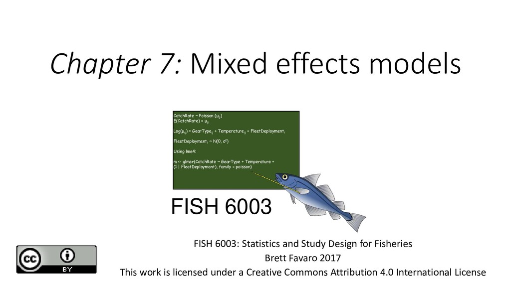
1. Chapter 7: Mixed effects models CatchRate ~ Poisson (μ ij ) E(CatchRate) = μ ij Log(μ ij ) = GearType ij + Temperature ij + FleetDeployment i FleetDeployment i ~ N(0, σ2) Using lme4: m <- glmer(CatchRate ~ GearType + Temperature + (1 | FleetDeployment), family = poisson) FISH 6003 FISH 6003: Statistics and Study Design for Fisheries Brett Favaro 2017 This work is licensed under a Creative Commons Attribution 4.0 International License
2. Land Acknowledgment We would like to respectfully acknowledge the territory in which we gather as the ancestral homelands of the Beothuk, and the island of Newfoundland as the ancestral homelands of the Mi’kmaq and Beothuk. We would also like to recognize the Inuit of Nunatsiavut and NunatuKavut and the Innu of Nitassinan, and their ancestors, as the original people of Labrador. We strive for respectful partnerships with all the peoples of this province as we search for collective healing and true reconciliation and honour this beautiful land together. http://www.mun.ca/aboriginal_affairs/
3. This week: • New terms: Fixed vs. Random effects • Introducing the Mixed Effects model
4. Consider a growth study… Treatment: Low food Medium food High food Feed them for six months Y: Size after six months Assume Y is continuous, normally distributed
5. Covariate: Food Response: Size Sizei = β0 + 0 * LowFood + β1 MedFood + β2 HighFood Also expressed as… Sizei ~ N(μi , σ2) E(Sizei ) = μi Var(Sizei ) = σ2 Sizei = β0 + FoodTreatmenti Low food Medium food High food
6. But there is a problem… Sizei ~ N(μi , σ2) E(Sizei ) = μi Var(Sizei ) = σ2 Sizei = β0 + FoodTreatmenti Low food Medium food High food Dependency structure: Fish in the same tank are more likely to be similar to each other, than to fish in other tanks! Pseudoreplication
7. Fix 1: Every fish gets a tank… Not cost-effective. Realistically, far fewer fish would be measured. Maybe appropriate for very small fish?
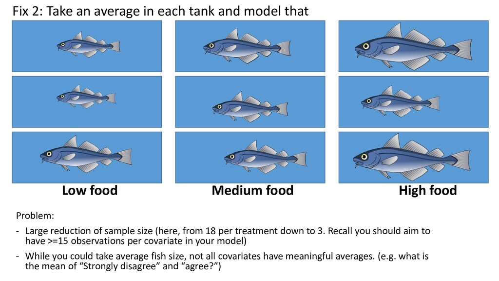
8. Low food Medium food High food Fix 2: Take an average in each tank and model that Problem: - Large reduction of sample size (here, from 18 per treatment down to 3. Recall you should aim to have >=15 observations per covariate in your model) - While you could take average fish size, not all covariates have meaningful averages. (e.g. what is the mean of “Strongly disagree” and “agree?”)
9. Low food Medium food High food Fix 3: Explicitly model tank-related effects as a random effect 1 2 3 4 5 6 7 8 9
10. Random Effect • Essentially a “grouping variable” • A categorical variable that imparts some sort of nesting structure into your data • Transects • “Strings” or “Fleets” of fishing gear • Individual identity (if you’re taking multiple observations from individuals) • A variable where either: • You don’t care about it, but need to include it to address dependency • You care about measuring the variance within different levels of the random effect • Not repeatable (i.e. “Tank 4” has no inherent, repeatable value) Fixed Effect • A variable with predetermined levels (or ranges) that is of direct interest. • All covariates we have used so far in the course have been fixed effects • E.g. • Age • Sex • Food treatment • Repeatable. (Male in this study meets an agreed-upon definition of male. Age 12 always means Age 12)
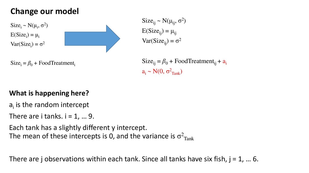
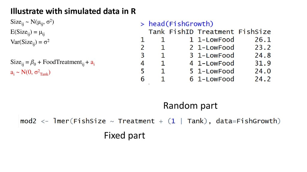
11. Sizei ~ N(μi , σ2) E(Sizei ) = μi Var(Sizei ) = σ2 Sizei = β0 + FoodTreatmenti Change our model What is happening here? ai is the random intercept There are i tanks. i = 1, … 9. Each tank has a slightly different y intercept. The mean of these intercepts is 0, and the variance is σ2 Tank There are j observations within each tank. Since all tanks have six fish, j = 1, … 6. Sizeij ~ N(μij , σ2) E(Sizeij ) = μij Var(Sizeij ) = σ2 Sizeij = β0 + FoodTreatmentij + ai ai ~ N(0, σ2 Tank )
12. Illustrate with simulated data in R Sizeij ~ N(μij , σ2) E(Sizeij ) = μij Var(Sizeij ) = σ2 Sizeij = β0 + FoodTreatmentij + ai ai ~ N(0, σ2 Tank ) Fixed part Random part
13. mod2 <- lmer(FishSize ~ Treatment + data = FishGrowth) (1 | Tank) A random intercept is shared by all individuals from the same tank
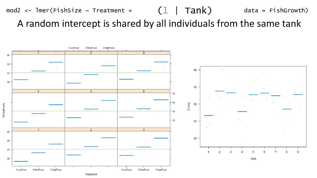
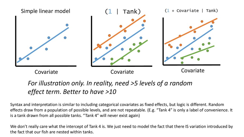
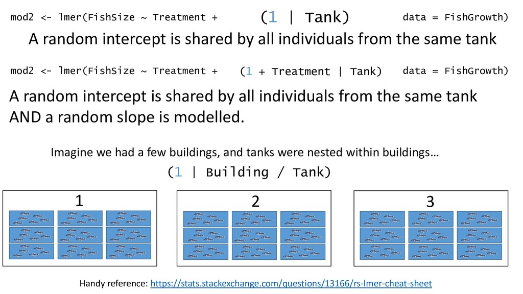
14. mod2 <- lmer(FishSize ~ Treatment + data = FishGrowth) (1 | Tank) A random intercept is shared by all individuals from the same tank mod2 <- lmer(FishSize ~ Treatment + data = FishGrowth) (1 + Treatment | Tank) A random intercept is shared by all individuals from the same tank AND a random slope is modelled. In this model, the shape of the relationship can differ in each tank
15. Simple linear model (1 | Tank) Covariate Covariate (1 + Covariate | Tank) Covariate For illustration only. In reality, need >5 levels of a random effect term. Better to have >10 Syntax and interpretation is similar to including categorical covariates as fixed effects, but logic is different. Random effects draw from a population of possible levels, and are not repeatable. (E.g. “Tank 4” is only a label of convenience. It is a tank drawn from all possible tanks. “Tank 4” will never exist again) We don’t really care what the intercept of Tank 4 is. We just need to model the fact that there IS variation introduced by the fact that our fish are nested within tanks.
16. mod2 <- lmer(FishSize ~ Treatment + data = FishGrowth) (1 | Tank) A random intercept is shared by all individuals from the same tank mod2 <- lmer(FishSize ~ Treatment + data = FishGrowth) (1 + Treatment | Tank) A random intercept is shared by all individuals from the same tank AND a random slope is modelled. Imagine we had a few buildings, and tanks were nested within buildings… 1 2 3 (1 | Building / Tank) Handy reference: https://stats.stackexchange.com/questions/13166/rs-lmer-cheat-sheet
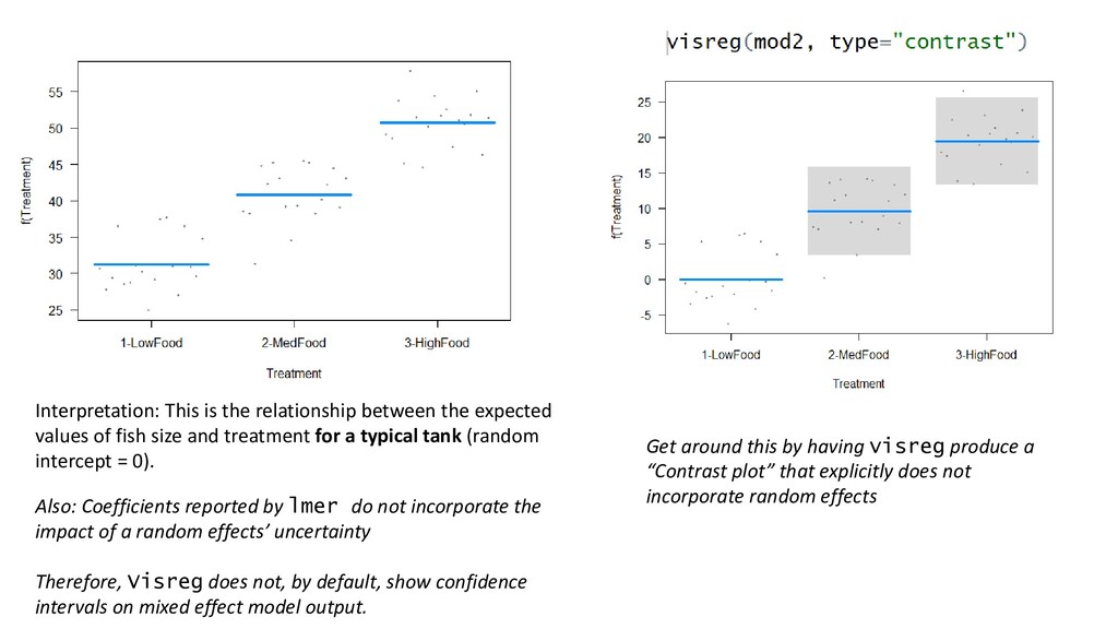
17. Also: Coefficients reported by lmer do not incorporate the impact of a random effects’ uncertainty Therefore, Visreg does not, by default, show confidence intervals on mixed effect model output. Get around this by having visreg produce a “Contrast plot” that explicitly does not incorporate random effects Interpretation: This is the relationship between the expected values of fish size and treatment for a typical tank (random intercept = 0).
19. Sizeij ~ N(μij , σ2) E(Sizeij ) = μij Var(Sizeij ) = σ2 Sizeij = β0 + FoodTreatmentij + ai ai ~ N(0, σ2 Tank ) Coefficients are reported for a typical tank, in the absence of tank- related effects
20. Sizeij ~ N(μij , 3.9102) E(Sizeij ) = μij Var(Sizeij ) = σ2 Sizeij = β0 + FoodTreatmentij + ai ai ~ N(0, 3.5062 Tank ) There are 54 fish within 9 tanks. 9 values for ai , normally distributed, with a mean of zero and a variance of 3.5062
21. The correlation between any two observations from the same tank is 0.445. That’s high – good evidence that you made the right choice in incorporating the random effect σ = 3.910 σTank = 3.506 Calculate the intraclass correlation 3.5062 ------------------- 3.5062 + 3.9102 = 0.445 If this value is 0 (i.e. there is no correlation within a class) then you could omit the random effect entirely. But better to not do that: If your study design should have a random effect, keep it in.
22. Where are the P-values?
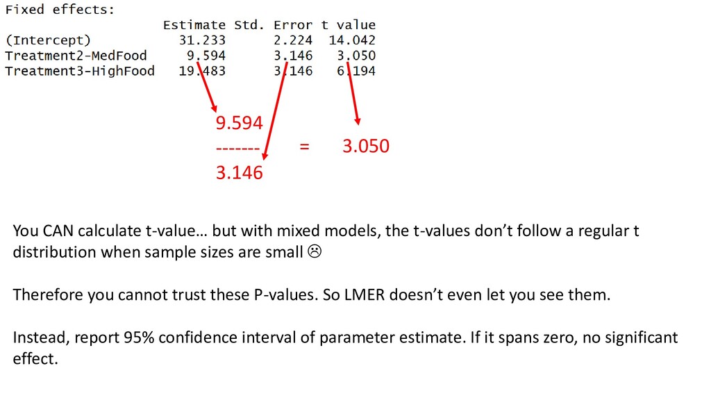
23. 9.594 ------- 3.146 3.050 = You CAN calculate t-value… but with mixed models, the t-values don’t follow a regular t distribution when sample sizes are small  Therefore you cannot trust these P-values. So LMER doesn’t even let you see them. Instead, report 95% confidence interval of parameter estimate. If it spans zero, no significant effect.
24. Recap • Fixed effect = a covariate of interest • Random effect = a covariate you need to include in your model to account for dependency structure • Random effects can address the problem of pseudoreplication • Use lme() or lmer()
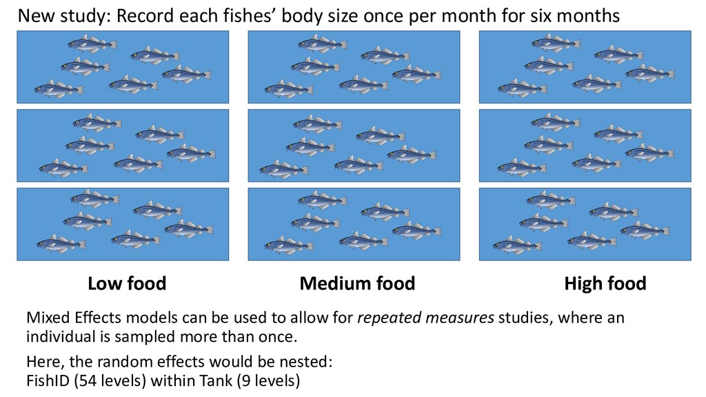
25. Low food Medium food High food New study: Record each fishes’ body size once per month for six months Mixed Effects models can be used to allow for repeated measures studies, where an individual is sampled more than once. Here, the random effects would be nested: FishID (54 levels) within Tank (9 levels)
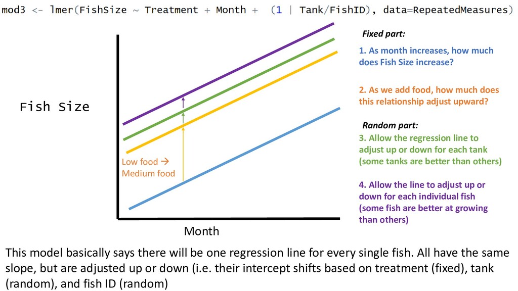
26. Fish Size Month 1. As month increases, how much does Fish Size increase? 2. As we add food, how much does this relationship adjust upward? Low food → Medium food 3. Allow the regression line to adjust up or down for each tank (some tanks are better than others) 4. Allow the line to adjust up or down for each individual fish (some fish are better at growing than others) This model basically says there will be one regression line for every single fish. All have the same slope, but are adjusted up or down (i.e. their intercept shifts based on treatment (fixed), tank (random), and fish ID (random) Fixed part: Random part:
27. • Random intercept model • Plots may look like this: • Thick line is “for a typical group” • Thin lines are regression lines for each specific group Zuur et al. 2010 • Random intercept, random slope model
28. Another application: Measurement Repeatability • There is always uncertainty around a measurement • Imagine we measured each fish twice. What is the measurement repeatability?
29. Can I use random effects in non-Gaussian GLMs? • Yes. See you in chapter 9…