FISH 6003: Week 6 - Generalized Linear Models

GLMS with count data

Transcript

1. Chapter 6: Generalized linear models CatchRate ~ Poisson (μ ij ) E(CatchRate) = μ ij Log(μ ij ) = GearType ij + Temperature ij + FleetDeployment i FleetDeployment i ~ N(0, σ2) Using lme4: m <- glmer(CatchRate ~ GearType + Temperature + (1 | FleetDeployment), family = poisson) FISH 6003 FISH 6003: Statistics and Study Design for Fisheries Brett Favaro 2017 This work is licensed under a Creative Commons Attribution 4.0 International License
2. Land Acknowledgment We would like to respectfully acknowledge the territory in which we gather as the ancestral homelands of the Beothuk, and the island of Newfoundland as the ancestral homelands of the Mi’kmaq and Beothuk. We would also like to recognize the Inuit of Nunatsiavut and NunatuKavut and the Innu of Nitassinan, and their ancestors, as the original people of Labrador. We strive for respectful partnerships with all the peoples of this province as we search for collective healing and true reconciliation and honour this beautiful land together. http://www.mun.ca/aboriginal_affairs/
3. This week: • Generalized Linear Models – how do they work? • Modelling: • Counts • Counts with lots of zeroes • Density, using offsets • Binomial
4. Recall: • Negative fitted values • Violation of homogeneity assumption • Simulation from model produces negative values Data: Huang et al (2017) εi ~ N(0, σ2) wrecksi = β0 + β1 hurricanesi + εi
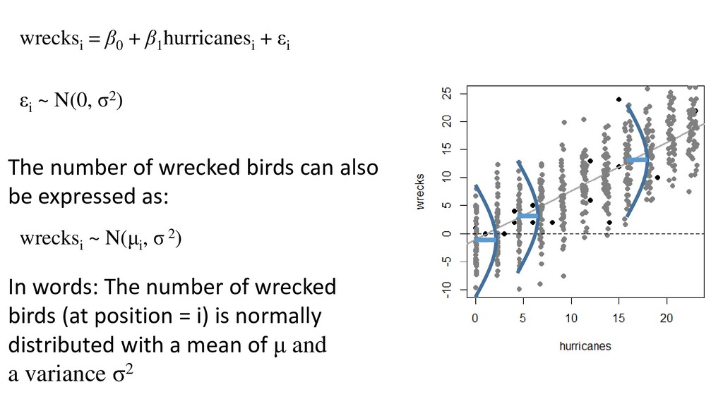
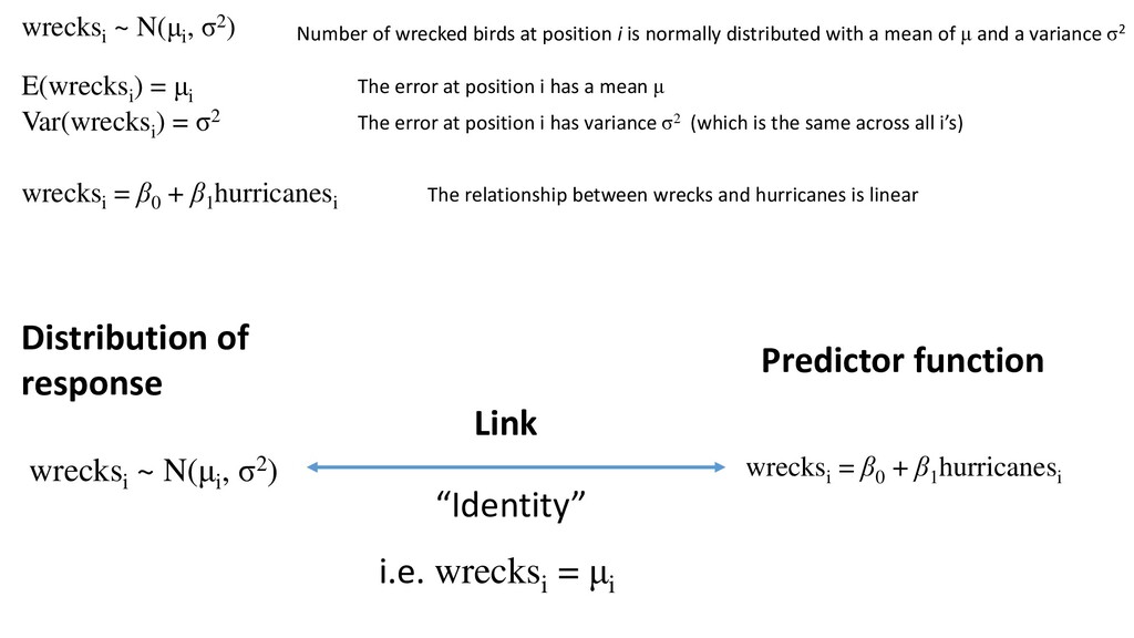
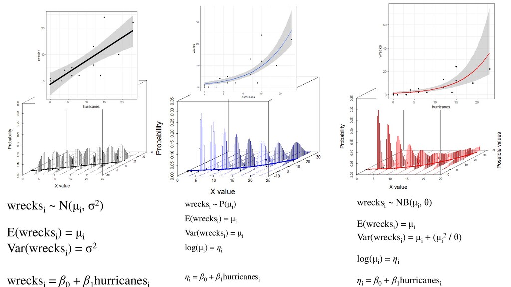
5. wrecksi = β0 + β1 hurricanesi + εi The number of wrecked birds can also be expressed as: wrecksi ~ N(μi , σ 2) εi ~ N(0, σ2) In words: The number of wrecked birds (at position = i) is normally distributed with a mean of μ and a variance σ2
6. wrecksi ~ N(μi , σ2) wrecksi = β0 + β1 hurricanesi Alternate view of model output
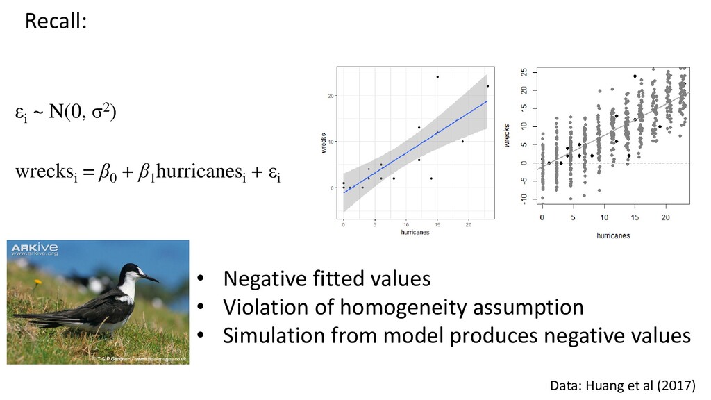
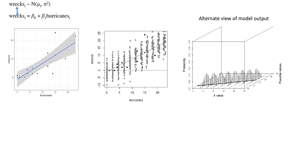
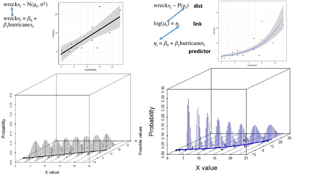
7. wrecksi ~ N(μi , σ2) E(wrecksi ) = μi Var(wrecksi ) = σ2 wrecksi = β0 + β1 hurricanesi Number of wrecked birds at position i is normally distributed with a mean of μ and a variance σ2 The error at position i has a mean μ The error at position i has variance σ2 (which is the same across all i’s) The relationship between wrecks and hurricanes is linear Distribution of response Predictor function wrecksi ~ N(μi , σ2) wrecksi = β0 + β1 hurricanesi Link “Identity” i.e. wrecksi = μi
8. Instead, let’s assume our response follows a Poisson distribution Poisson distributions are: - Defined only by a mean (lambda) - Bound at zero 1000 samples from populations with Poisson distributions:
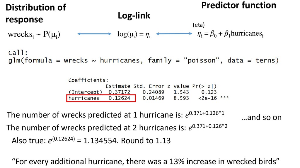
9. Distribution of response Predictor function wrecksi ~ P(μi ) ηi = β0 + β1 hurricanesi Link (eta) log(μi ) = ηi μi = eηi μi = eβ0 + β1 hurricanesi log-link function (default) Notes: - No more assumption of equal variance (Poisson distribution has just one parameter) - Fitted values will never be negative - Still a linear model
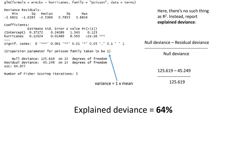
10. Distribution of response Predictor function wrecksi ~ P(μi ) ηi = β0 + β1 hurricanesi Log-link (eta) log(μi ) = ηi The number of wrecks predicted at 1 hurricane is: e0.371+0.126*1 The number of wrecks predicted at 2 hurricanes is: e0.371+0.126*2 …and so on Also true: e(0.12624) = 1.134554. Round to 1.13 “For every additional hurricane, there was a 13% increase in wrecked birds”
11. Predictor function wrecksi ~ N(μi , σ2) wrecksi = β0 + β1 hurricanesi Link “Identity” Distribution of response wrecksi ~ P(μi ) ηi = β0 + β1 hurricanesi log(μi ) = ηi β1 = 0.87 (95% C.I. 0.49 – 1.24) For every additional hurricane, there were 0.87 (95% CI: 0.49 – 1.24) more wrecked birds β1 = 0.13 (95% C.I. 0.10 – 0.16) For every additional hurricane, there were 13% (95% CI: 10 – 16%) more wrecked birds
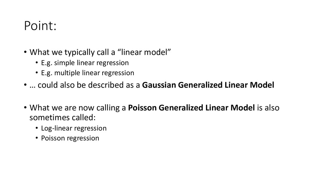
12. Point: • What we typically call a “linear model” • E.g. simple linear regression • E.g. multiple linear regression • … could also be described as a Gaussian Generalized Linear Model • What we are now calling a Poisson Generalized Linear Model is also sometimes called: • Log-linear regression • Poisson regression
13. wrecksi ~ N(μi , σ2) wrecksi = β0 + β1 hurricanesi
14. wrecksi ~ N(μi , σ2) wrecksi = β0 + β1 hurricanesi wrecksi ~ P(μi ) ηi = β0 + β1 hurricanesi log(μi ) = ηi In Poisson distributions, mean = variance
15. wrecksi ~ N(μi , σ2) wrecksi = β0 + β1 hurricanesi wrecksi ~ P(μi ) ηi = β0 + β1 hurricanesi log(μi ) = ηi link dist predictor
16. How are parameters estimated? • In Gaussian model: Ordinary least squares • In GLM: Maximum Likelihood Good to read about it. But not necessary to understand it to interpret model output, or assess fit.
17. Here, there’s no such thing as R2. Instead, report explained deviance: Null deviance – Residual deviance -------------------------------------------- Null deviance 125.619 – 45.249 ----------------------- 125.619 Explained deviance = 64% variance = 1 x mean
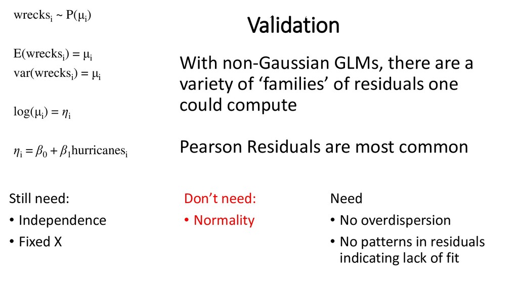
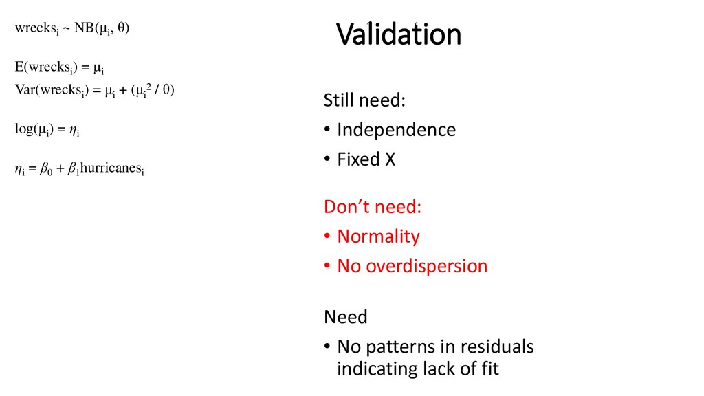
18. wrecksi ~ P(μi ) E(wrecksi ) = μi var(wrecksi ) = μi log(μi ) = ηi ηi = β0 + β1 hurricanesi Validation Still need: • Independence • Fixed X With non-Gaussian GLMs, there are a variety of ‘families’ of residuals one could compute Pearson Residuals are most common Don’t need: • Normality Need • No overdispersion • No patterns in residuals indicating lack of fit
19. Residuals No patterns in residuals indicating lack of fit Plot: - Residuals vs. covariates in model - Residuals vs. covariates NOT in model - Residuals vs. time and space - Residuals vs. fitted values Residuals
20. wrecksi ~ P(μi ) E(wrecksi ) = μi var(wrecksi ) = μi ηi = β0 + β1 hurricanesi Overdispersion Need: • Independence • Fixed X • No overdispersion • No patterns in residuals indicating lack of fit Dispersion statistic: Sum of squared Pearson residuals --------------------------------------------- Residual degrees of freedom (aka, # observations N - # parameters p) Dispersion statistic = 1 → perfect > 1 → Overdispersed  (common) < 1 → Underdispersed (rare)
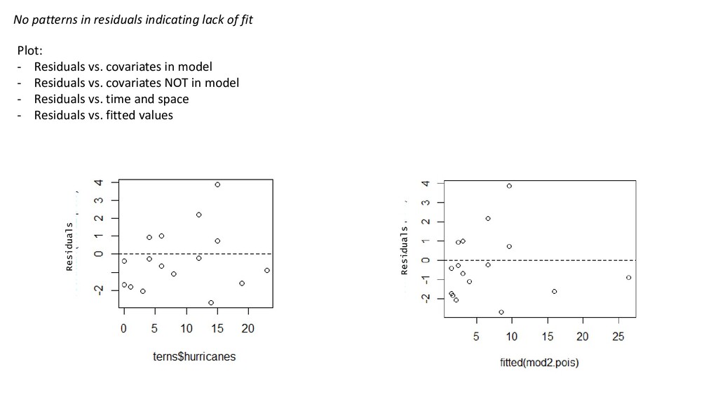
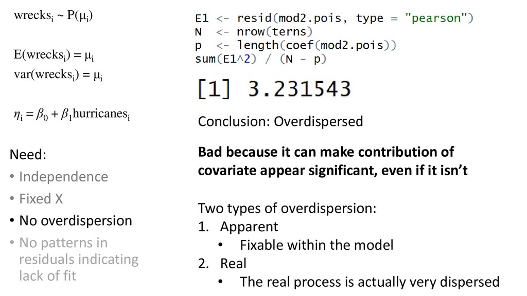
21. wrecksi ~ P(μi ) E(wrecksi ) = μi var(wrecksi ) = μi ηi = β0 + β1 hurricanesi Need: • Independence • Fixed X • No overdispersion • No patterns in residuals indicating lack of fit Conclusion: Overdispersed Two types of overdispersion: 1. Apparent • Fixable within the model 2. Real • The real process is actually very dispersed Bad because it can make contribution of covariate appear significant, even if it isn’t
22. Sources of apparent overdispersion (Zuur et al. 2009): 1. Outliers in Y 2. Missing covariates 3. Missing interactions 4. Zero-inflation 5. Dependency not accounted for 6. Non-linear patterns 7. Wrong link function Solutions Rule each of these out. Wrong choice = biased parameters 1. Remove 2. Add 3. Add 4. Use Zero-Inflated model (later) 5. Add a ‘random effect’ (later) 6. Use a Generalized Additive Model (not this course) 7. Change it
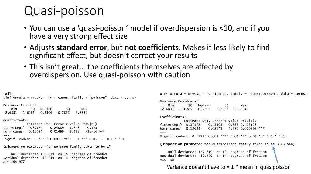
23. Quasi-poisson • You can use a ‘quasi-poisson’ model if overdispersion is <10, and if you have a very strong effect size • Adjusts standard error, but not coefficients. Makes it less likely to find significant effect, but doesn’t correct your results • This isn’t great… the coefficients themselves are affected by overdispersion. Use quasi-poisson with caution Variance doesn’t have to = 1 * mean in quasipoisson
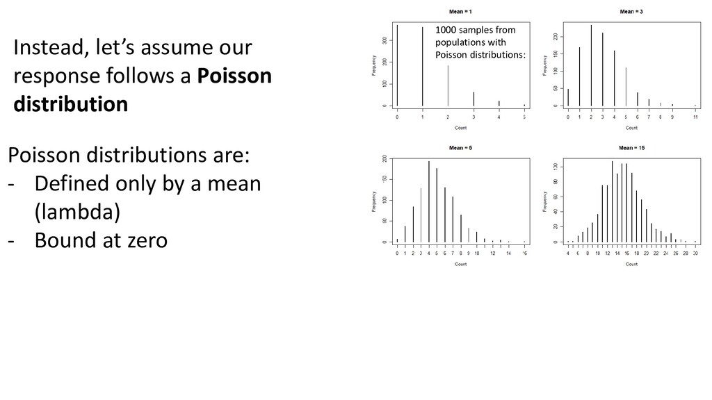
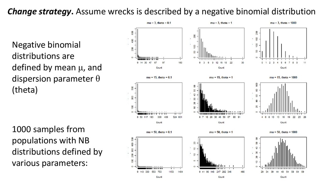
24. Change strategy. Assume wrecks is described by a negative binomial distribution Negative binomial distributions are defined by mean μ, and dispersion parameter θ (theta) 1000 samples from populations with NB distributions defined by various parameters:
25. Predictor function ηi = β0 + β1 hurricanesi Link (eta) log(μi ) = ηi wrecksi ~ P(μi ) Distribution of response wrecksi ~ N(μi , σ2) wrecksi = β0 + β1 hurricanesi “Identity” wrecksi ~ NB(μi , θ) log(μi ) = ηi ηi = β0 + β1 hurricanesi (theta) wrecksi ~ NB(μi , θ) E(wrecksi ) = μi Var(wrecksi ) = μi + (μi 2 / θ) log(μi ) = ηi ηi = β0 + β1 hurricanesi
26. wrecksi ~ P(μi ) ηi = β0 + β1 hurricanesi log(μi ) = ηi link dist predictor wrecksi ~ NB(μi , θ) ηi = β0 + β1 hurricanesi log(μi ) = ηi
27. Validation Still need: • Independence • Fixed X Don’t need: • Normality • No overdispersion Need • No patterns in residuals indicating lack of fit wrecksi ~ NB(μi , θ) E(wrecksi ) = μi Var(wrecksi ) = μi + (μi 2 / θ) log(μi ) = ηi ηi = β0 + β1 hurricanesi
28. Residuals No patterns in residuals indicating lack of fit Plot: - Residuals vs. covariates in model - Residuals vs. covariates NOT in model - Residuals vs. time and space - Residuals vs. fitted values Residuals
29. Here, there’s no such thing as R2. Instead, report explained deviance: Null deviance – Residual deviance -------------------------------------------- Null deviance 47.678 – 17.129 ----------------------- 47.678 Explained deviance = 62%
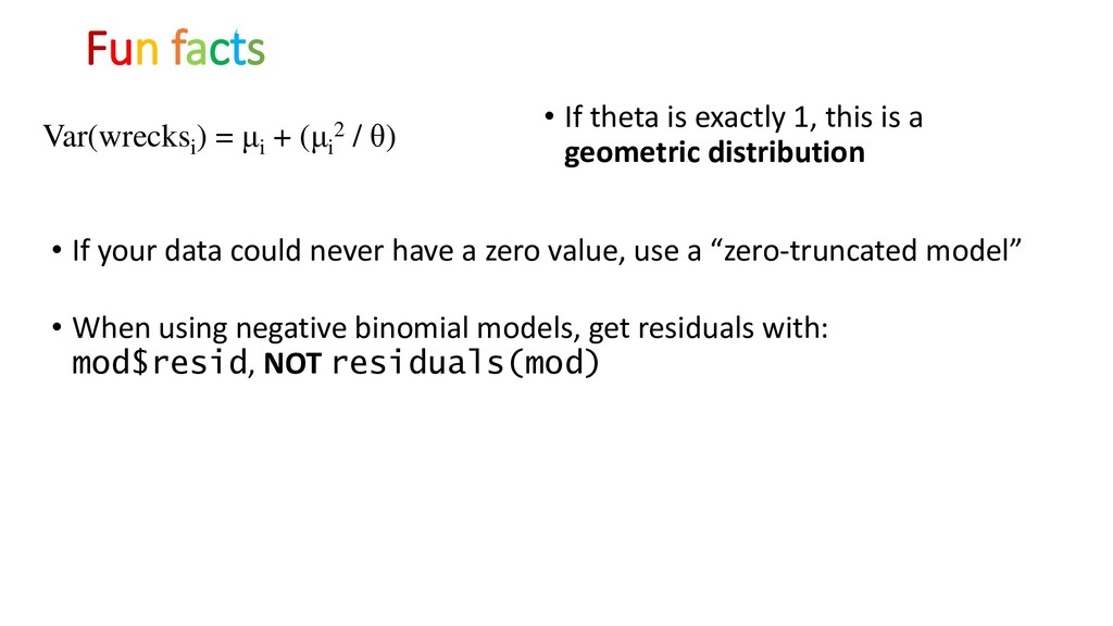
30. Fun facts • If theta is exactly 1, this is a geometric distribution Var(wrecksi ) = μi + (μi 2 / θ) • If your data could never have a zero value, use a “zero-truncated model” • When using negative binomial models, get residuals with: mod$resid, NOT residuals(mod)
31. wrecksi ~ N(μi , σ2) E(wrecksi ) = μi Var(wrecksi ) = σ2 wrecks = β + β hurricanes wrecksi ~ P(μi ) E(wrecksi ) = μi Var(wrecksi ) = μi log(μi ) = ηi ηi = β0 + β1 hurricanesi wrecksi ~ NB(μi , θ) E(wrecksi ) = μi Var(wrecksi ) = μi + (μi 2 / θ) log(μi ) = ηi ηi = β0 + β1 hurricanesi
32. Gaussian Poisson Negative Binomial The NB model is best here because: - Model passes the ‘sanity test’ (no negative fitted values) - No model assumptions are clearly violated Let’s interpret!
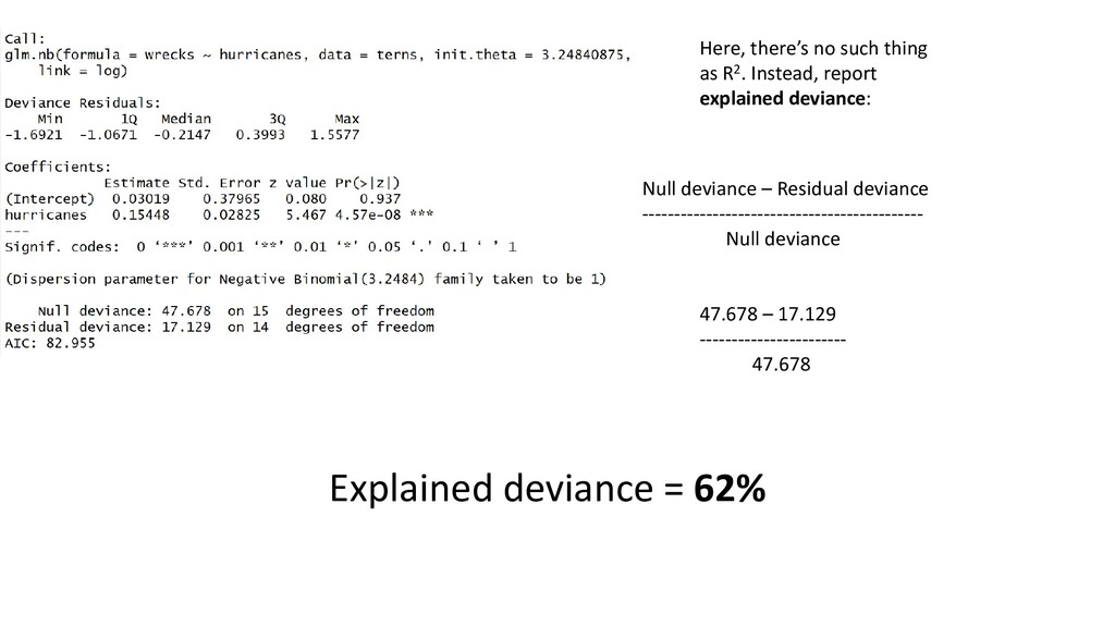
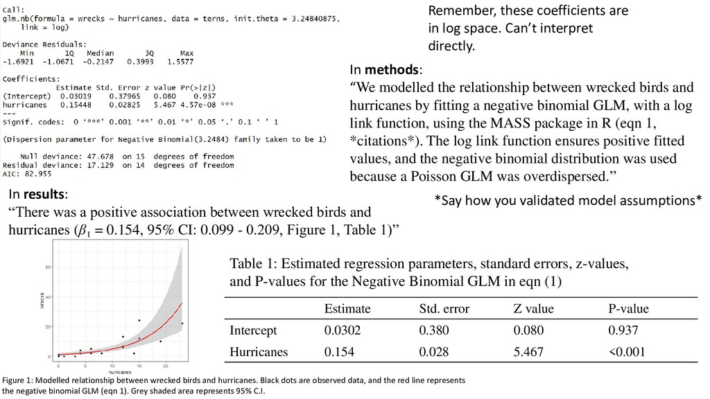
33. Remember, these coefficients are in log space. Can’t interpret directly. In results: “There was a positive association between wrecked birds and hurricanes (β1 = 0.154, 95% CI: 0.099 - 0.209, Figure 1, Table 1)” Figure 1: Modelled relationship between wrecked birds and hurricanes. Black dots are observed data, and the red line represents the negative binomial GLM (eqn 1). Grey shaded area represents 95% C.I. Estimate Std. error Z value P-value Intercept 0.0302 0.380 0.080 0.937 Hurricanes 0.154 0.028 5.467 <0.001 Table 1: Estimated regression parameters, standard errors, z-values, and P-values for the Negative Binomial GLM in eqn (1) In methods: “We modelled the relationship between wrecked birds and hurricanes by fitting a negative binomial GLM, with a log link function, using the MASS package in R (eqn 1, *citations*). The log link function ensures positive fitted values, and the negative binomial distribution was used because a Poisson GLM was overdispersed.” *Say how you validated model assumptions*
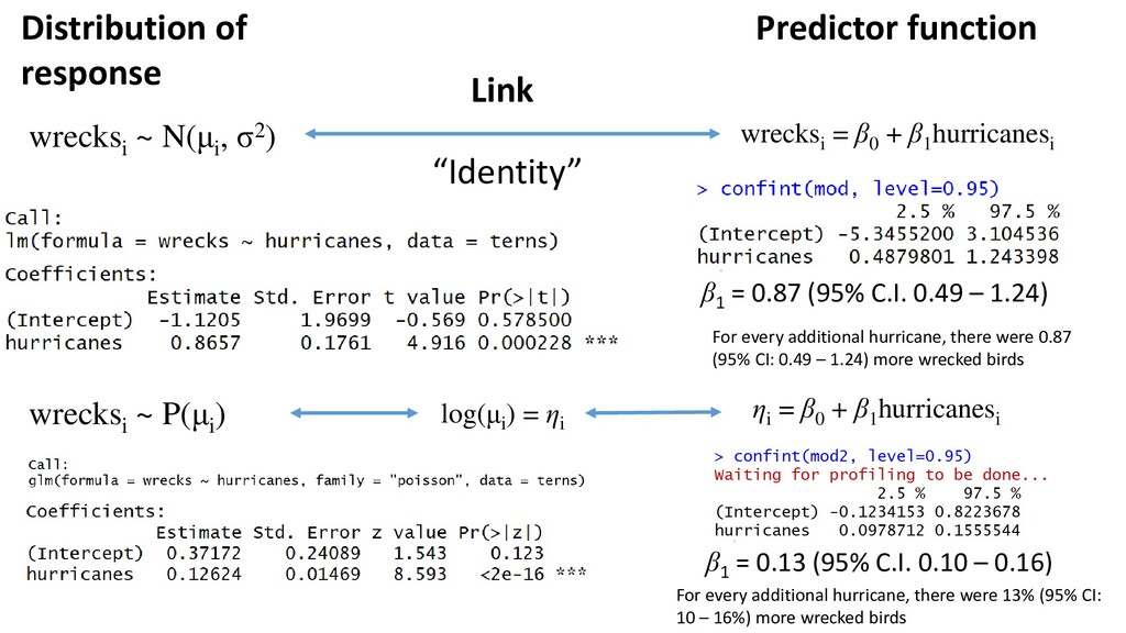
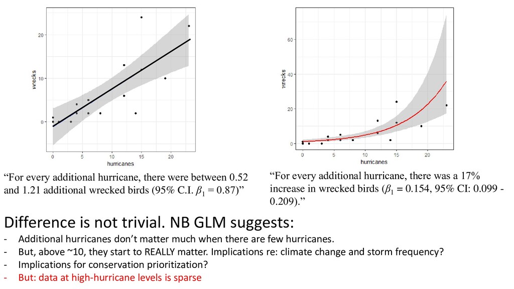
34. “For every additional hurricane, there were between 0.52 and 1.21 additional wrecked birds (95% C.I. β1 = 0.87)” “For every additional hurricane, there was a 17% increase in wrecked birds (β1 = 0.154, 95% CI: 0.099 - 0.209).” Difference is not trivial. NB GLM suggests: - Additional hurricanes don’t matter much when there are few hurricanes. - But, above ~10, they start to REALLY matter. Implications re: climate change and storm frequency? - Implications for conservation prioritization? - But: data at high-hurricane levels is sparse
35. Let’s do all this together: Run through Exercise 1 as a class
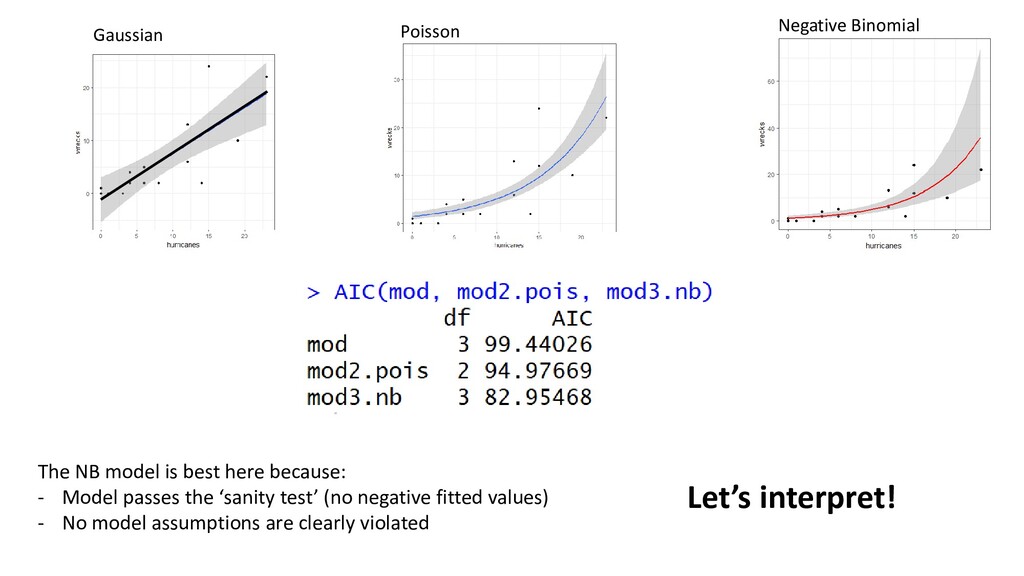
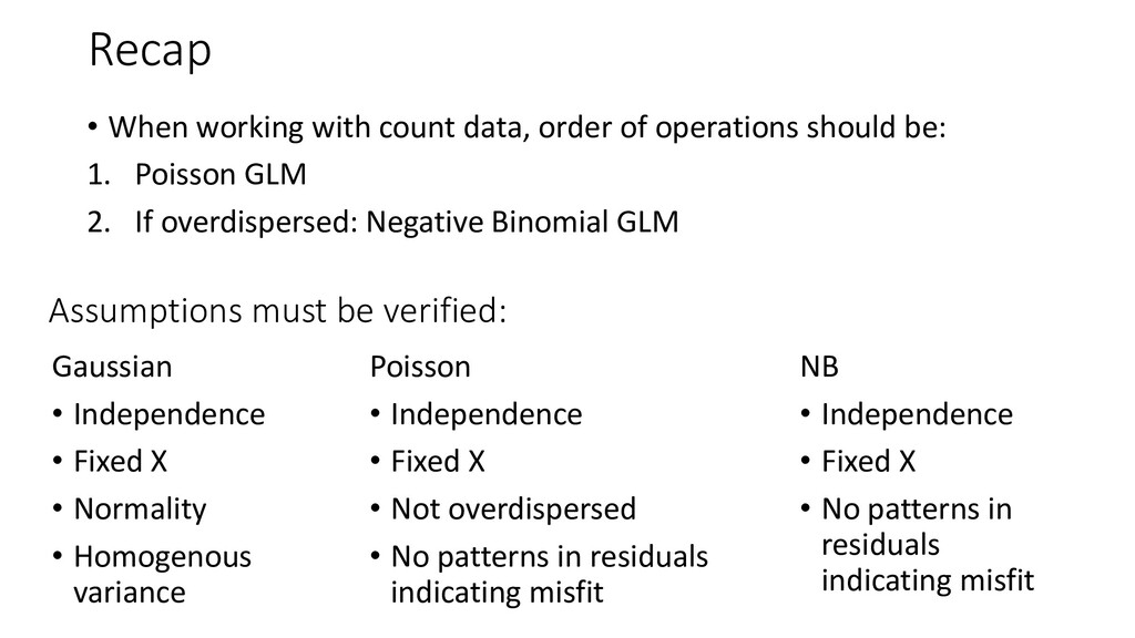
36. Recap • When working with count data, order of operations should be: 1. Poisson GLM 2. If overdispersed: Negative Binomial GLM Assumptions must be verified: NB • Independence • Fixed X • No patterns in residuals indicating misfit Gaussian • Independence • Fixed X • Normality • Homogenous variance Poisson • Independence • Fixed X • Not overdispersed • No patterns in residuals indicating misfit
37. Density – Count data in disguise! • If we have density data, we are really modelling: • Count / Area • Count / Volume • Let’s return to the Lionfish example…
38. Go to R Code: Exercise 2 After R code: Our model now looks like this: Because: Count ------------------------------------------ = e^(β + β*Covariate) Area/Effort/Other denominator Algebra Count = e^(β + β*Covariate + ln(Denominator))
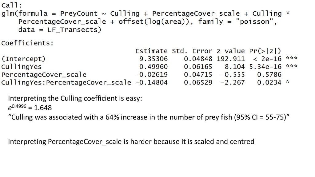
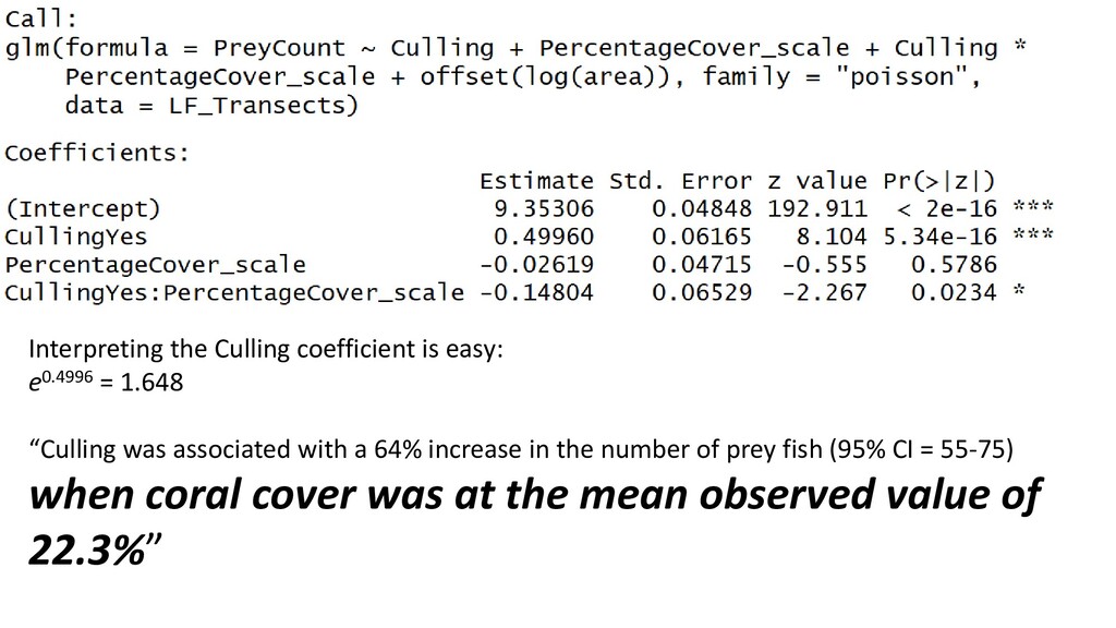
39. Interpreting the Culling coefficient is easy: e0.4996 = 1.648 “Culling was associated with a 64% increase in the number of prey fish (95% CI = 55-75)” Interpreting PercentageCover_scale is harder because it is scaled and centred
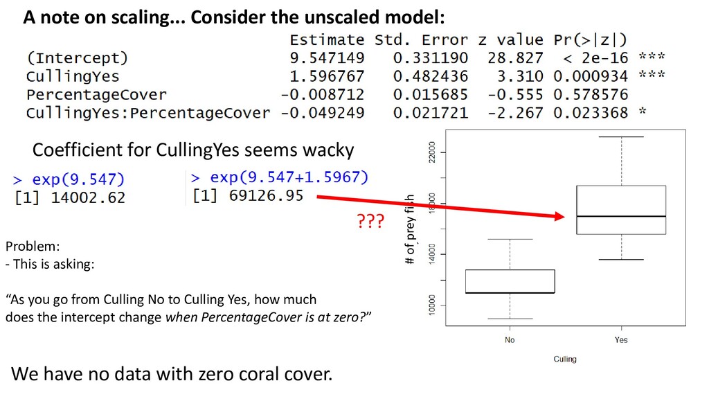
40. A note on scaling... Consider the unscaled model: # of prey fish Coefficient for CullingYes seems wacky ??? Problem: - This is asking: “As you go from Culling No to Culling Yes, how much does the intercept change when PercentageCover is at zero?” We have no data with zero coral cover.
41. Unscaled: The model does work. But when interpreting the impact of culling on prey, you would need to make sure to add enough “percentage cover” units for this to be a reasonable interpretation. “At a median value for PercentageCover, a one-unit increase in Culling increases prey fish density by…” The Visreg package (http://pbreheny.github.io/visreg/glm.html) can assist here
42. Interpreting the Culling coefficient is easy: e0.4996 = 1.648 “Culling was associated with a 64% increase in the number of prey fish (95% CI = 55-75) when coral cover was at the mean observed value of 22.3%”
43. General rule: • All model selection, validation, etc. should be done on the scale in which the modelling occurred. • Interpretation, visualization, etc. should be done in reality.
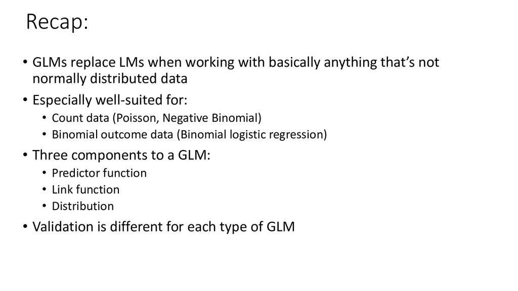
44. • GLMs replace LMs when working with basically anything that’s not normally distributed data • Especially well-suited for: • Count data (Poisson, Negative Binomial) • Binomial outcome data (Binomial logistic regression) • Three components to a GLM: • Predictor function • Link function • Distribution • Validation is different for each type of GLM Recap:
45. • Next week: • GLM for Proportional data • Multinomial logistic regression (for nominal Y) • Cumulative logistic regression (for ordinal Y)