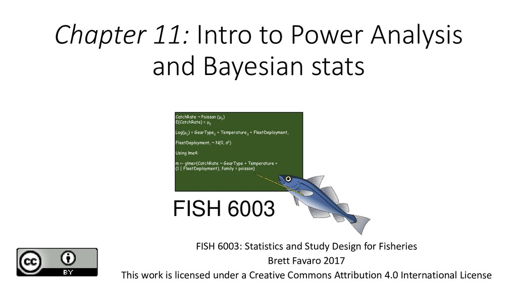
~ Poisson (μ ij ) E(CatchRate) = μ ij Log(μ ij ) = GearType ij + Temperature ij + FleetDeployment i FleetDeployment i ~ N(0, σ2) Using lme4: m <- glmer(CatchRate ~ GearType + Temperature + (1 | FleetDeployment), family = poisson) FISH 6003 FISH 6003: Statistics and Study Design for Fisheries Brett Favaro 2017 This work is licensed under a Creative Commons Attribution 4.0 International License
in which we gather as the ancestral homelands of the Beothuk, and the island of Newfoundland as the ancestral homelands of the Mi’kmaq and Beothuk. We would also like to recognize the Inuit of Nunatsiavut and NunatuKavut and the Innu of Nitassinan, and their ancestors, as the original people of Labrador. We strive for respectful partnerships with all the peoples of this province as we search for collective healing and true reconciliation and honour this beautiful land together. http://www.mun.ca/aboriginal_affairs/
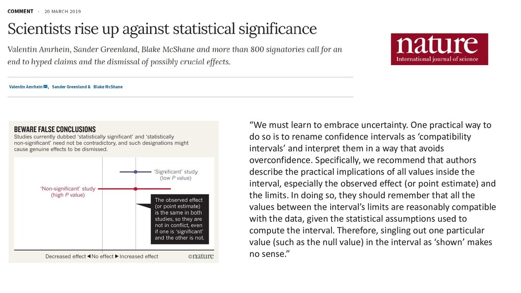
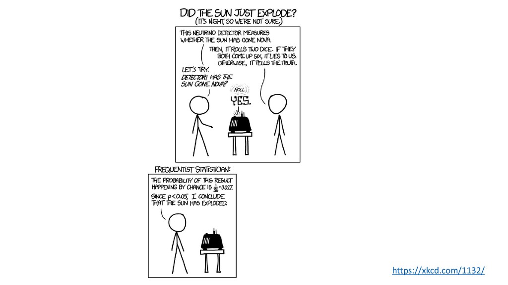
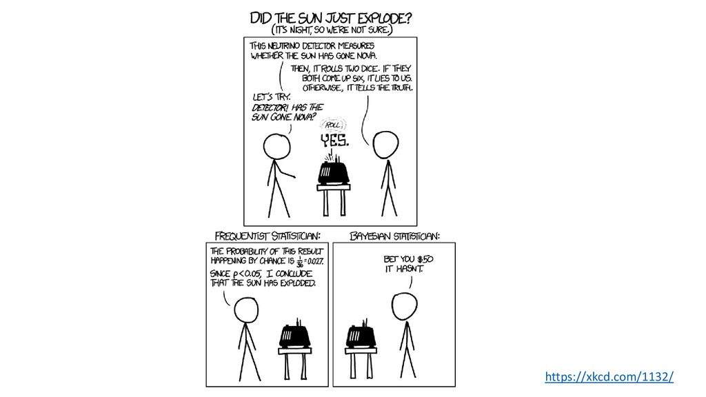
do so is to rename confidence intervals as ‘compatibility intervals’ and interpret them in a way that avoids overconfidence. Specifically, we recommend that authors describe the practical implications of all values inside the interval, especially the observed effect (or point estimate) and the limits. In doing so, they should remember that all the values between the interval’s limits are reasonably compatible with the data, given the statistical assumptions used to compute the interval. Therefore, singling out one particular value (such as the null value) in the interval as ‘shown’ makes no sense.”
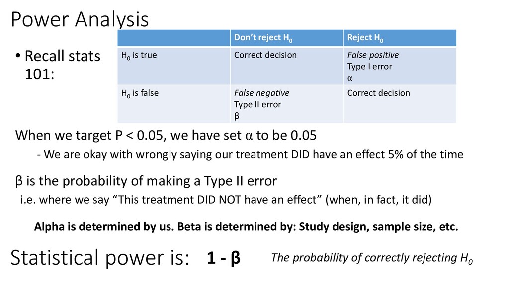
H0 H0 is true Correct decision False positive Type I error α H0 is false False negative Type II error β Correct decision When we target P < 0.05, we have set α to be 0.05 β is the probability of making a Type II error - We are okay with wrongly saying our treatment DID have an effect 5% of the time i.e. where we say “This treatment DID NOT have an effect” (when, in fact, it did) Alpha is determined by us. Beta is determined by: Study design, sample size, etc. Statistical power is: 1 - β The probability of correctly rejecting H0
of group A and B... Type 1 Error: Reject Ho and conclude there is an effect, but there actually is no effect. The probability of this error is denoted by α (usually set to 0.05) Type 2 Error: Accept Ho and conclude there is no effect, but there actually is an effect. The probability of this error is denoted by β Statistical power is 1 – β, and is the probability of correctly rejecting Ho An experiment with high β has low power.
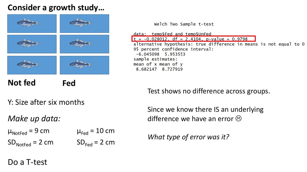
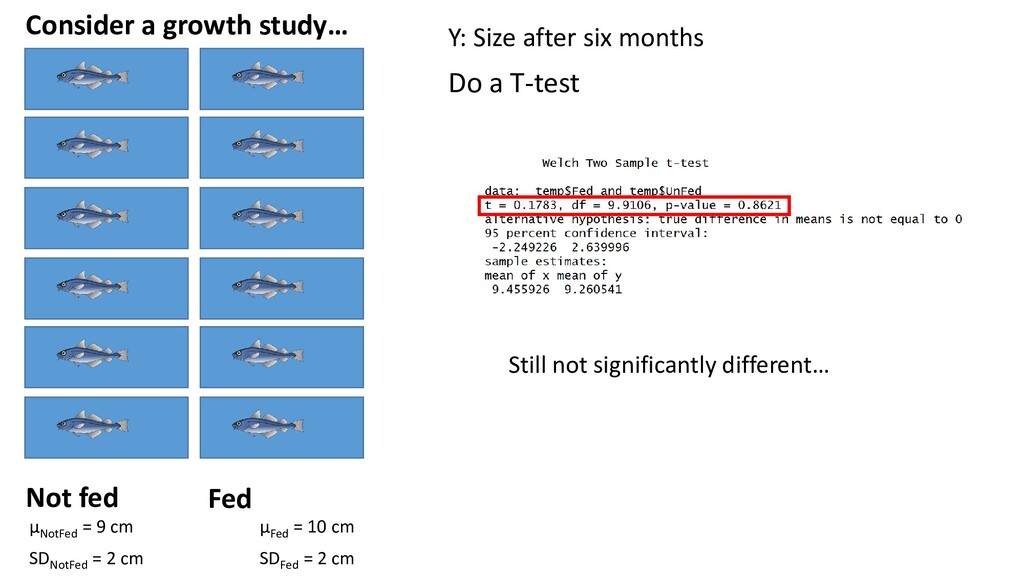
a T-test Not fed Fed Make up data: μNotFed = 9 cm μFed = 10 cm SDNotFed = 2 cm SDFed = 2 cm Test shows no difference across groups. Since we know there IS an underlying difference we have an error What type of error was it?
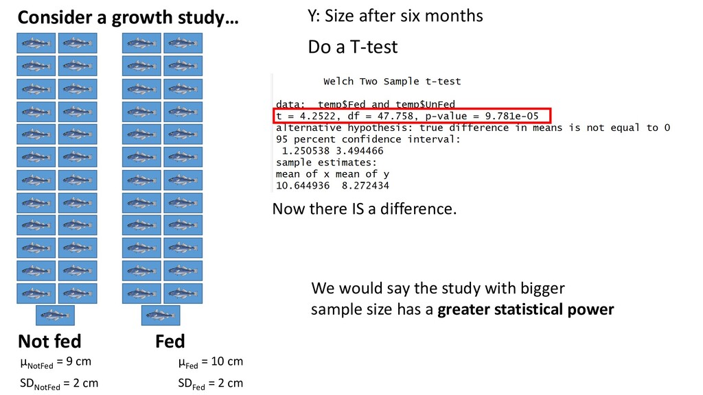
a T-test Not fed Fed μNotFed = 9 cm μFed = 10 cm SDNotFed = 2 cm SDFed = 2 cm Now there IS a difference. We would say the study with bigger sample size has a greater statistical power
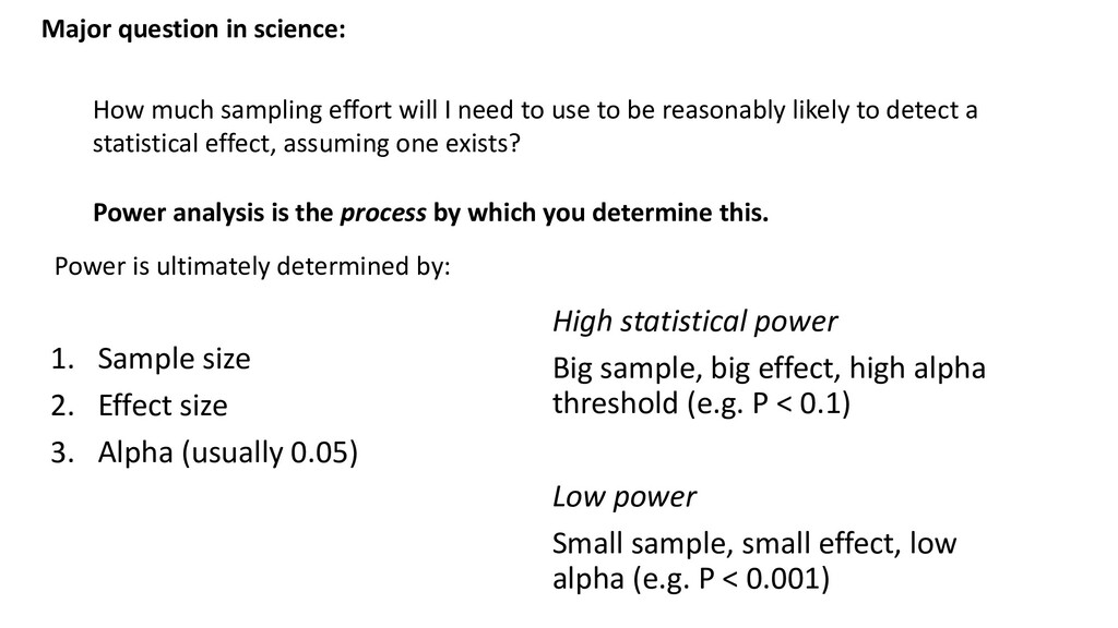
need to use to be reasonably likely to detect a statistical effect, assuming one exists? Power analysis is the process by which you determine this. Power is ultimately determined by: 1. Sample size 2. Effect size 3. Alpha (usually 0.05) High statistical power Big sample, big effect, high alpha threshold (e.g. P < 0.1) Low power Small sample, small effect, low alpha (e.g. P < 0.001)
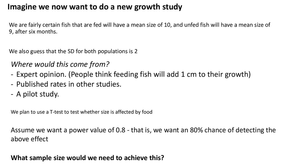
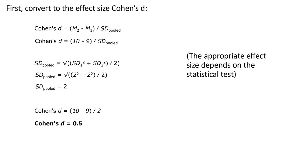
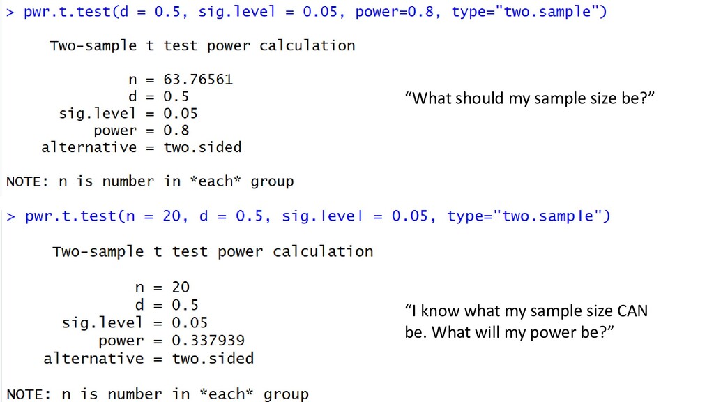
We are fairly certain fish that are fed will have a mean size of 10, and unfed fish will have a mean size of 9, after six months. We also guess that the SD for both populations is 2 Where would this come from? - Expert opinion. (People think feeding fish will add 1 cm to their growth) - Published rates in other studies. - A pilot study. Assume we want a power value of 0.8 - that is, we want an 80% chance of detecting the above effect What sample size would we need to achieve this? We plan to use a T-test to test whether size is affected by food
to be 80% likely to detect this affect, given an effect size of 0.5 and sample size of 20?” Rare “How big would the effect size need to be, for me to have an 80% chance of detecting it, given a sample size of 20?”
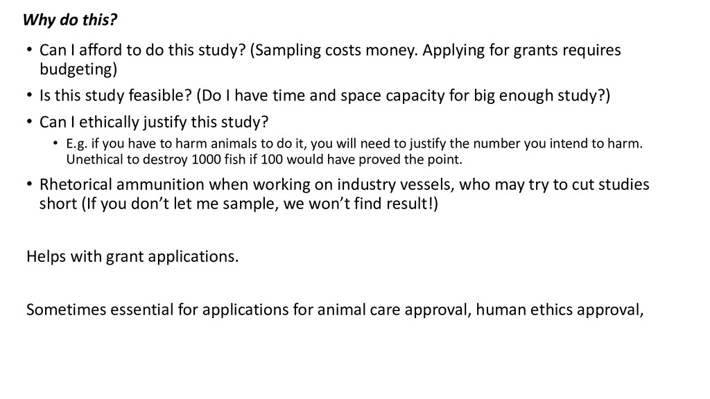
study? (Sampling costs money. Applying for grants requires budgeting) • Is this study feasible? (Do I have time and space capacity for big enough study?) • Can I ethically justify this study? • E.g. if you have to harm animals to do it, you will need to justify the number you intend to harm. Unethical to destroy 1000 fish if 100 would have proved the point. • Rhetorical ammunition when working on industry vessels, who may try to cut studies short (If you don’t let me sample, we won’t find result!) Helps with grant applications. Sometimes essential for applications for animal care approval, human ethics approval,
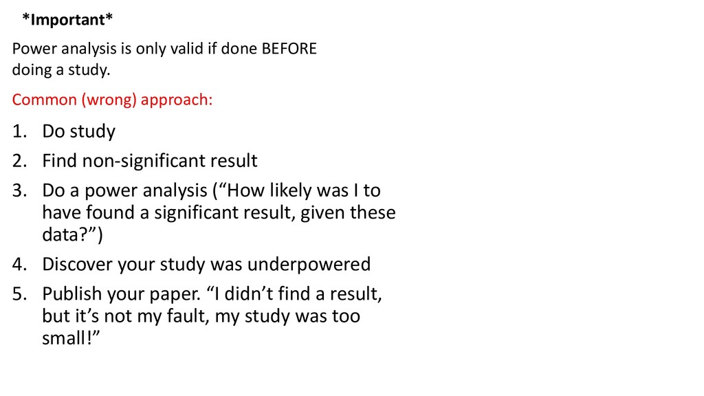
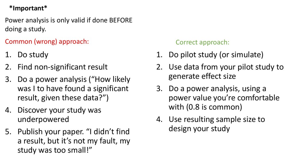
a study. Common (wrong) approach: 1. Do study 2. Find non-significant result 3. Do a power analysis (“How likely was I to have found a significant result, given these data?”) 4. Discover your study was underpowered 5. Publish your paper. “I didn’t find a result, but it’s not my fault, my study was too small!”
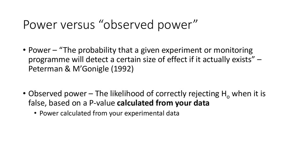
a given experiment or monitoring programme will detect a certain size of effect if it actually exists” – Peterman & M’Gonigle (1992) • Observed power – The likelihood of correctly rejecting Ho when it is false, based on a P-value calculated from your data • Power calculated from your experimental data
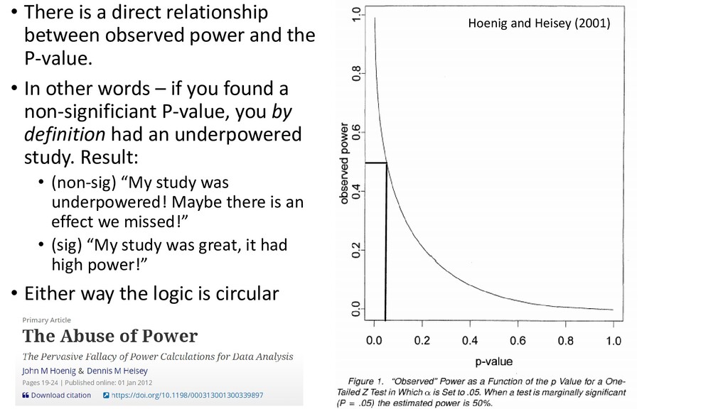
the P-value. • In other words – if you found a non-significiant P-value, you by definition had an underpowered study. Result: • (non-sig) “My study was underpowered! Maybe there is an effect we missed!” • (sig) “My study was great, it had high power!” • Either way the logic is circular Hoenig and Heisey (2001)
a study. Common (wrong) approach: 1. Do study 2. Find non-significant result 3. Do a power analysis (“How likely was I to have found a significant result, given these data?”) 4. Discover your study was underpowered 5. Publish your paper. “I didn’t find a result, but it’s not my fault, my study was too small!” Correct approach: 1. Do pilot study (or simulate) 2. Use data from your pilot study to generate effect size 3. Do a power analysis, using a power value you’re comfortable with (0.8 is common) 4. Use resulting sample size to design your study
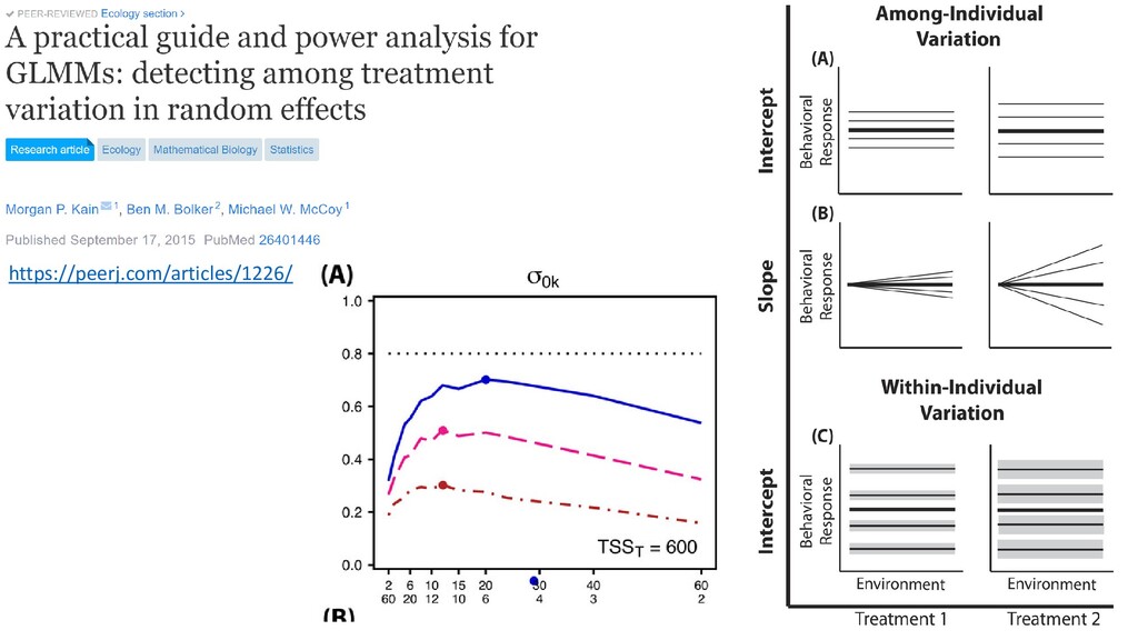
power analysis is logically harder • Link function • Many covariates and interactions • Random effects • Whereas in simple models you simply specify ¾ parameters, and solve for the last, with GLMMs it is not so simple • Need to simulate many realizations of a model, and see how those models change as variance increases, covariates change, etc. • Short answer: It can be done, but it’s more challenging
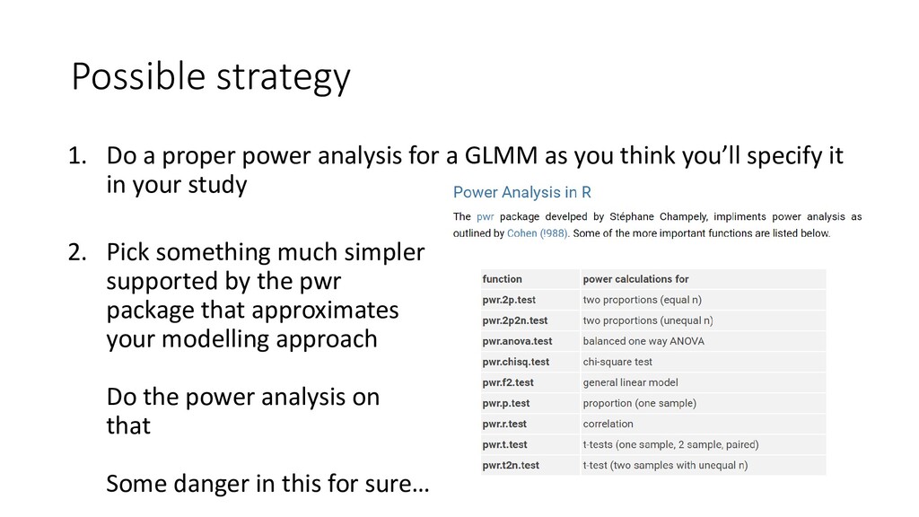
GLMM as you think you’ll specify it in your study 2. Pick something much simpler supported by the pwr package that approximates your modelling approach Do the power analysis on that Some danger in this for sure…
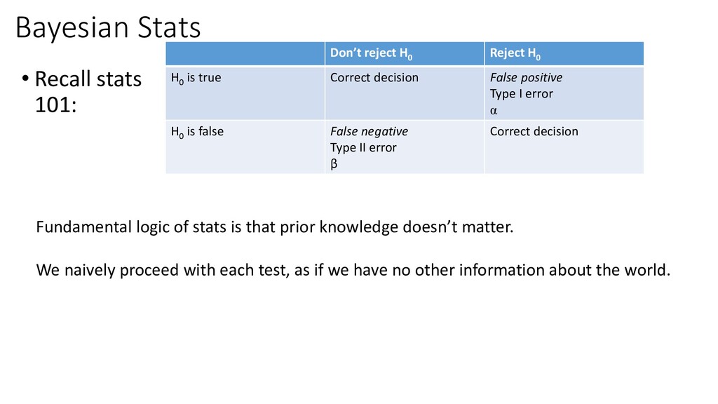
H0 H0 is true Correct decision False positive Type I error α H0 is false False negative Type II error β Correct decision Fundamental logic of stats is that prior knowledge doesn’t matter. We naively proceed with each test, as if we have no other information about the world.
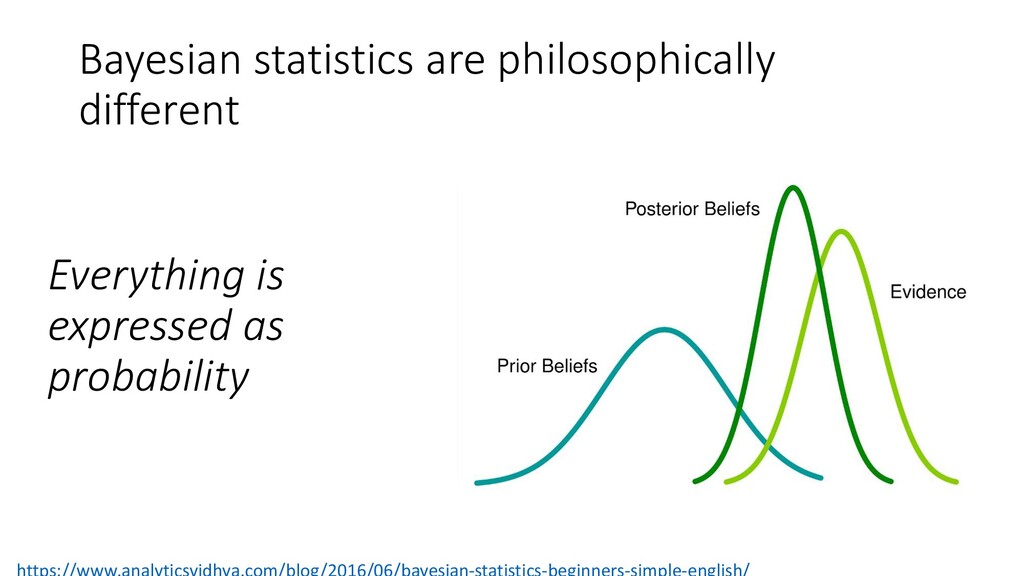
given what we already know to be true In Bayesian statistics, we incorporate prior information in our analysis. Good Bad Frequentist stats assume infinite replication of studies. That’s fictional. Models are no longer strictly objective. What constitutes “prior knowledge?” and how do we defend using it? Makes intuitive sense. If we KNOW something, why NOT use it? What values, specifically, should we use for priors? (starts big fights) Why is this good/bad?
not easily explained by a frequentist GLMM – e.g. the distribution does not match any supported by a mainstream package • There is spatial or temporal dependency where prior knowledge matters • E.g. you know for sure that a species CAN’T exist below a certain depth. Good to incorporate that prior information into the model