ij ) E(CatchRate) = μ ij Log(μ ij ) = GearType ij + Temperature ij + FleetDeployment i FleetDeployment i ~ N(0, σ2) Using lme4: m <- glmer(CatchRate ~ GearType + Temperature + (1 | FleetDeployment), family = poisson) FISH 6003 FISH 6003: Statistics and Study Design for Fisheries Brett Favaro
in which we gather as the ancestral homelands of the Beothuk, and the island of Newfoundland as the ancestral homelands of the Mi’kmaq and Beothuk. We would also like to recognize the Inuit of Nunatsiavut and NunatuKavut and the Innu of Nitassinan, and their ancestors, as the original people of Labrador. We strive for respectful partnerships with all the peoples of this province as we search for collective healing and true reconciliation and honour this beautiful land together. http://www.mun.ca/aboriginal_affairs/
a variable of interest distorts a relationship for which you are testing • COLLINEARITY: Variables in a model that are highly correlated with each other Y: Swimming speed Y: Swimming speed Covariates: Body size, body weight Puig-Pons (2018) X: Body size Major influence, not measured or modelled: Temperature
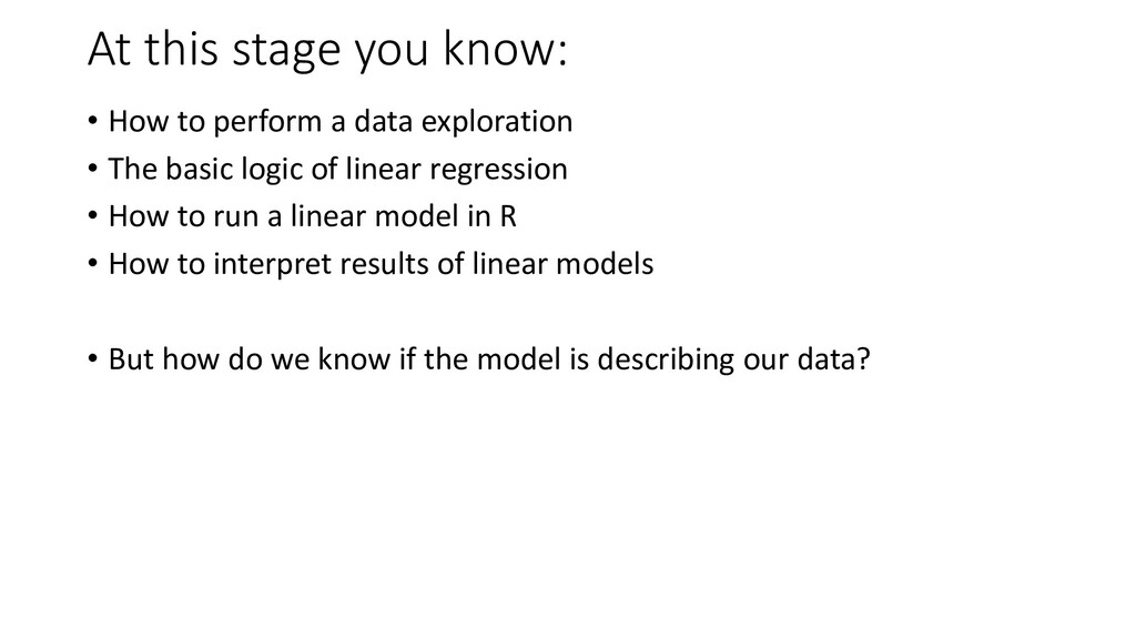
data exploration • The basic logic of linear regression • How to run a linear model in R • How to interpret results of linear models • But how do we know if the model is describing our data?
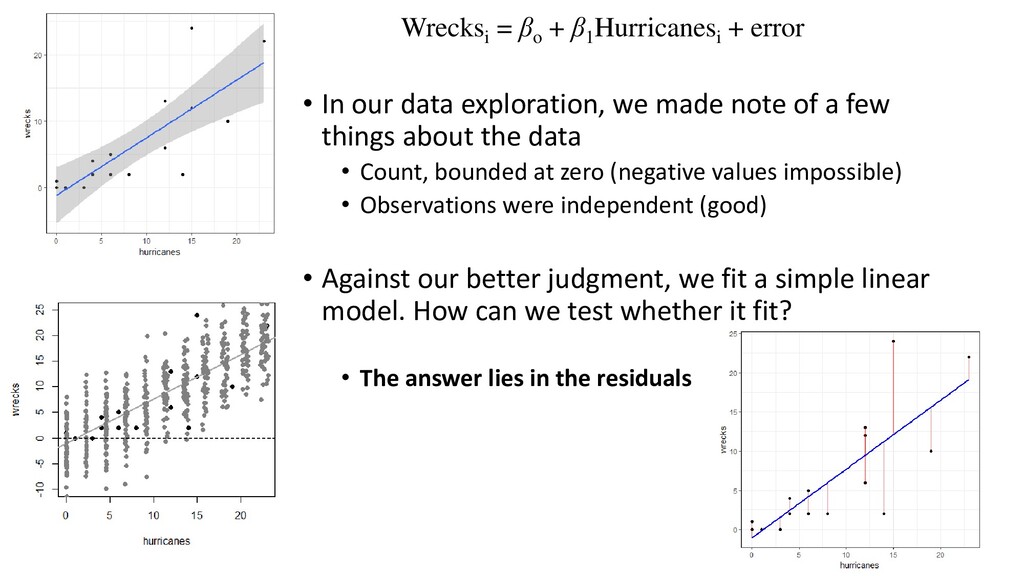
our data exploration, we made note of a few things about the data • Count, bounded at zero (negative values impossible) • Observations were independent (good) • Against our better judgment, we fit a simple linear model. How can we test whether it fit? • The answer lies in the residuals
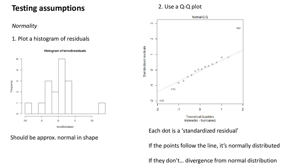
Use a Q-Q plot Should be approx. normal in shape Each dot is a ‘standardized residual’ If the points follow the line, it’s normally distributed If they don’t… divergence from normal distribution
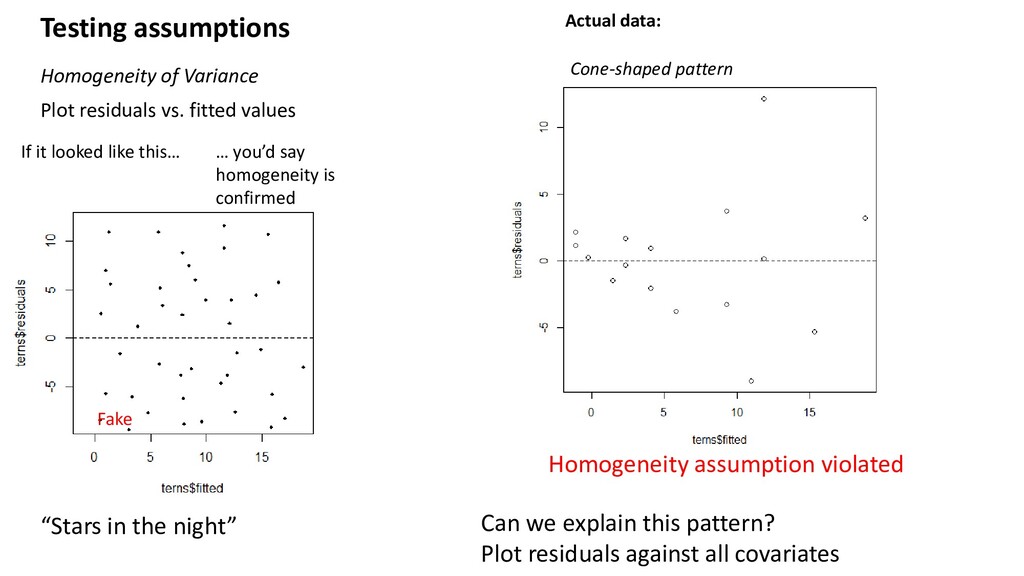
If it looked like this… Fake “Stars in the night” Homogeneity assumption violated Actual data: Cone-shaped pattern … you’d say homogeneity is confirmed Can we explain this pattern? Plot residuals against all covariates
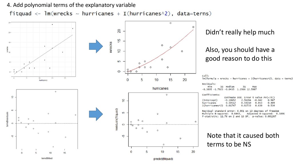
missing a covariate or polynomial term - Model fit is very poor at high values - Lots of low values, fewer high values (probably need a GLM, negative binomial distribution. Come back later)
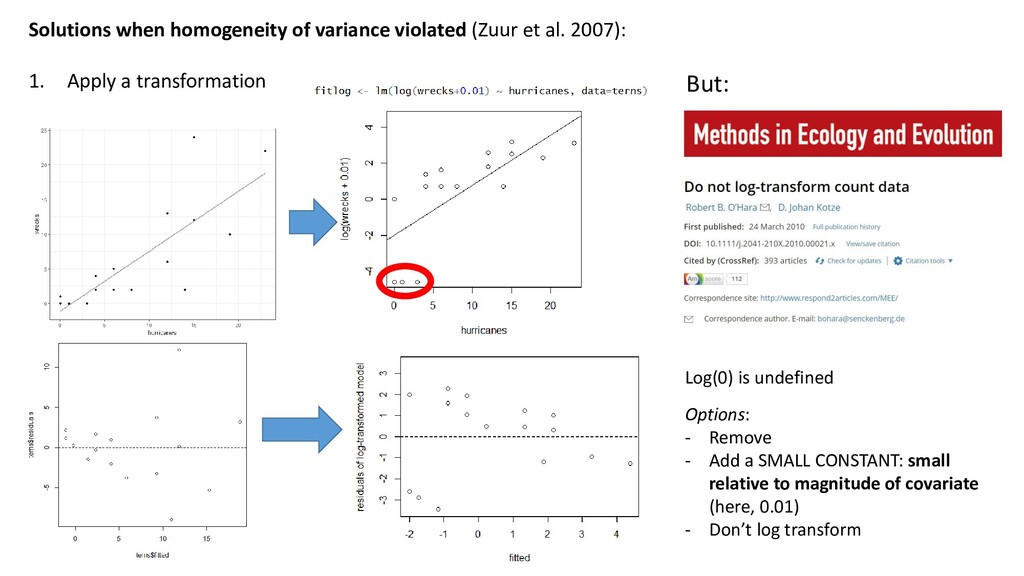
1. Apply a transformation But: Log(0) is undefined Options: - Remove - Add a SMALL CONSTANT: small relative to magnitude of covariate (here, 0.01) - Don’t log transform
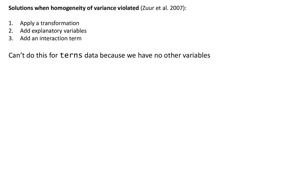
1. Apply a transformation 2. Add explanatory variables 3. Add an interaction term 4. Add a polynomial 5. Fit a generalized linear model (later this course) 6. Fit a mixed model (later this course) 7. Fit a generalized additive model (Another course) 8. Allow for variance to change using generalized least squares (Another course) Don’t just try these randomly. Models are used to describe reality. You should have an a priori reason for applying a solution above: Not just “to improve model fit.”
looking at the study design We can also assess it by looking at residuals versus each covariate Here, we have just the one covariate But… things to watch out for: Temporal correlation Model misfit (e.g. influential covariate missing from the model)
pseudoreplication - Incorporate study design in model - E.g. If observations nested within ~ 5 or fewer “Sites” incorporate “Site” as a covariate - If more than 10 levels of “Site,” make it a ‘random effect’ term (come back in a few weeks) - E.g. If time series data, compute an “autocorrelation function” (Not sure if we will do this in the present course) - Extreme cases: If the study design is too flawed, give up. Descriptive stats and qualitative descriptions only Violation due to model misfit - Specify a new model - Include additional explanatory variables - Come back in GLM lecture
positions are accurate? If not… solution is beyond the scope of what we’re doing here. Try to avoid this problem by: - Designing a good study - Minimizing the number of steps between data collection and analysis - Recall the lionfish paper (Week 4), where the covariate was biomass per hectare. Uncertainty existed in: - Count of fish - Length of fish (visual estimate) - Length-weight relationship curve (more uncertainty added going from length → weight) - Converting count to density (due to estimation of transect area) - Instead, use the actual counts, thus eliminating three sources of X variation
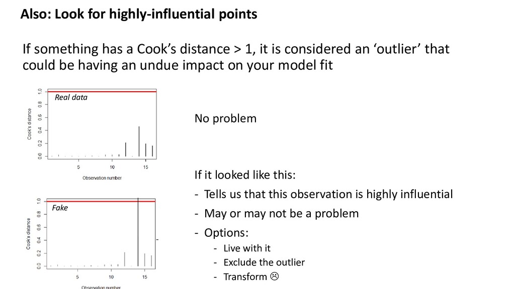
distance > 1, it is considered an ‘outlier’ that could be having an undue impact on your model fit Real data Fake No problem If it looked like this: - Tells us that this observation is highly influential - May or may not be a problem - Options: - Live with it - Exclude the outlier - Transform
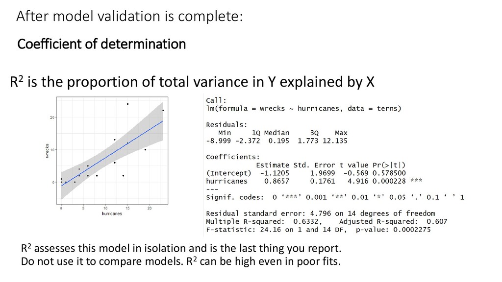
the proportion of total variance in Y explained by X R2 assesses this model in isolation and is the last thing you report. Do not use it to compare models. R2 can be high even in poor fits.
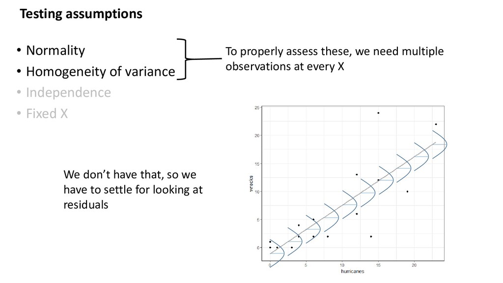
• Independence • Fixed X Test with: - Histogram of residuals, qqplot - Plot residuals vs fitted values - Common sense, plot residuals vs. covariates (those in the model, and those not) - Common sense If these are violated… - Some things can be dealt with statistically (transform, add a covariate, etc.) - Some things cannot (study design) - Document all decisions (including “ignore”)
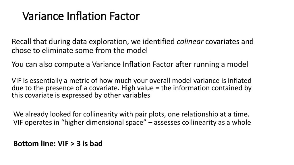
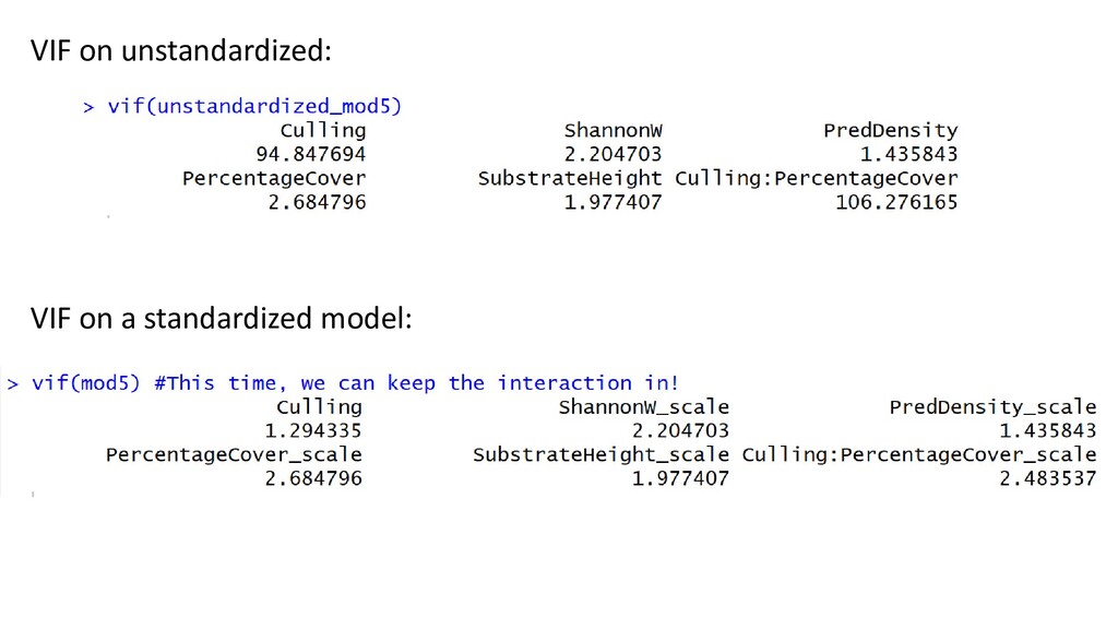
colinear covariates and chose to eliminate some from the model You can also compute a Variance Inflation Factor after running a model Bottom line: VIF > 3 is bad VIF is essentially a metric of how much your overall model variance is inflated due to the presence of a covariate. High value = the information contained by this covariate is expressed by other variables We already looked for collinearity with pair plots, one relationship at a time. VIF operates in “higher dimensional space” – assesses collinearity as a whole
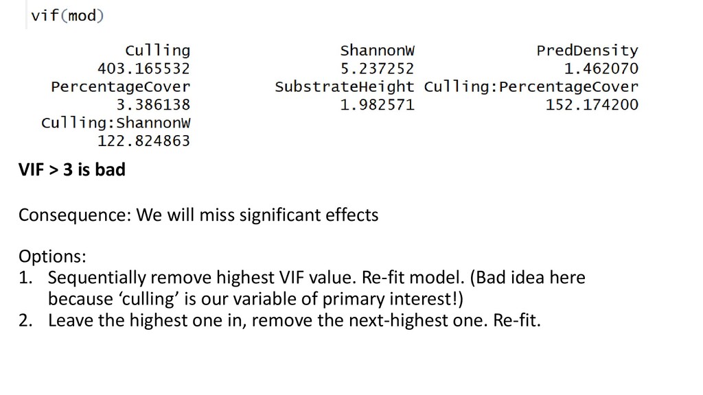
VIF value. Re-fit model. (Bad idea here because ‘culling’ is our variable of primary interest!) 2. Leave the highest one in, remove the next-highest one. Re-fit. Consequence: We will miss significant effects
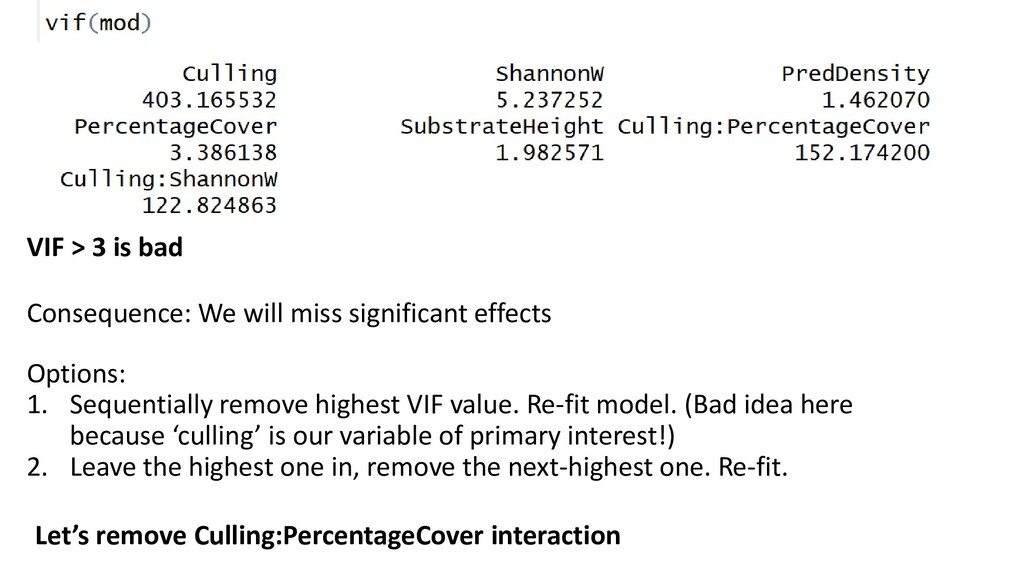
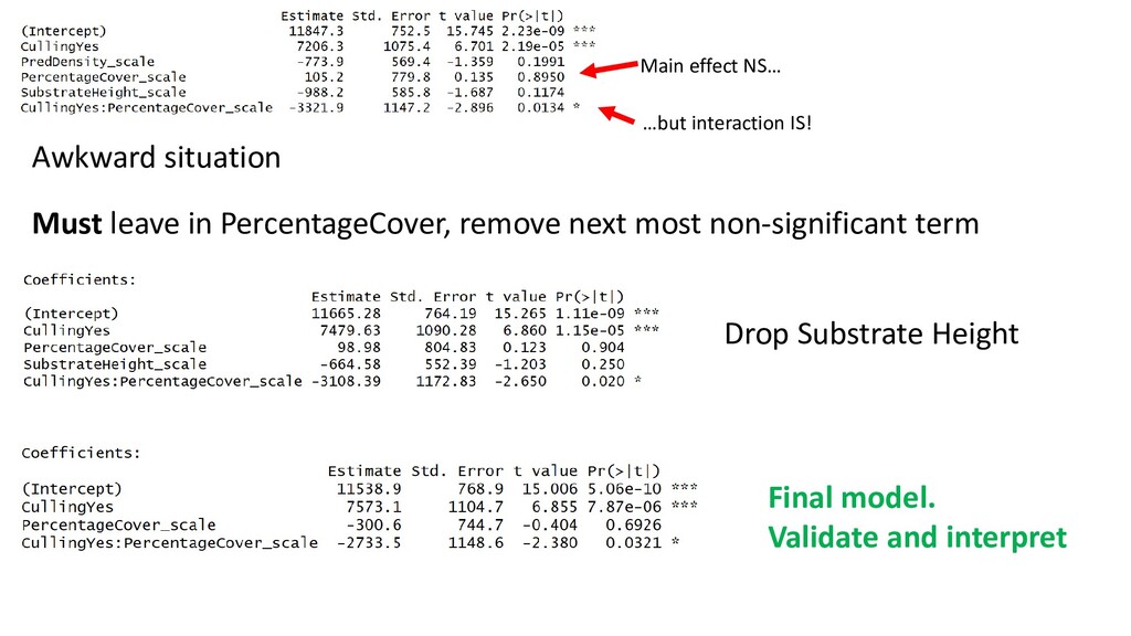
VIF value. Re-fit model. (Bad idea here because ‘culling’ is our variable of primary interest!) 2. Leave the highest one in, remove the next-highest one. Re-fit. Consequence: We will miss significant effects Let’s remove Culling:PercentageCover interaction
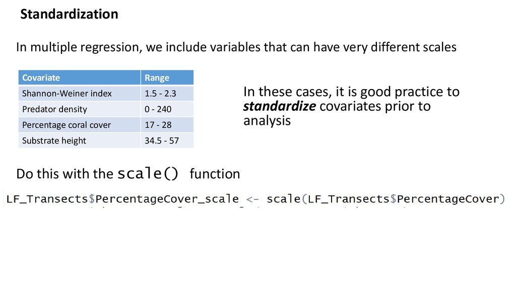
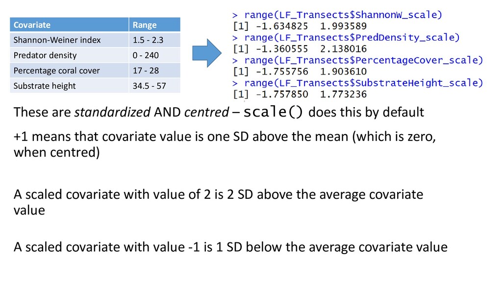
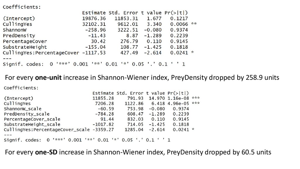
very different scales Covariate Range Shannon-Weiner index 1.5 - 2.3 Predator density 0 - 240 Percentage coral cover 17 - 28 Substrate height 34.5 - 57 In these cases, it is good practice to standardize covariates prior to analysis Do this with the scale() function
- 240 Percentage coral cover 17 - 28 Substrate height 34.5 - 57 These are standardized AND centred – scale() does this by default +1 means that covariate value is one SD above the mean (which is zero, when centred) A scaled covariate with value of 2 is 2 SD above the average covariate value A scaled covariate with value -1 is 1 SD below the average covariate value
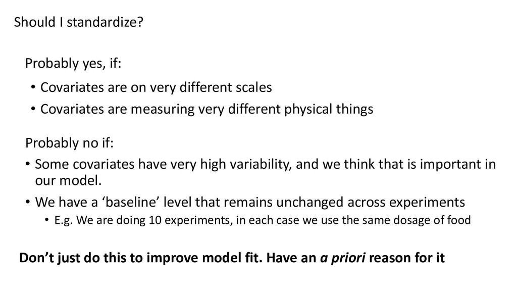
very different scales • Covariates are measuring very different physical things Probably no if: • Some covariates have very high variability, and we think that is important in our model. • We have a ‘baseline’ level that remains unchanged across experiments • E.g. We are doing 10 experiments, in each case we use the same dosage of food Don’t just do this to improve model fit. Have an a priori reason for it
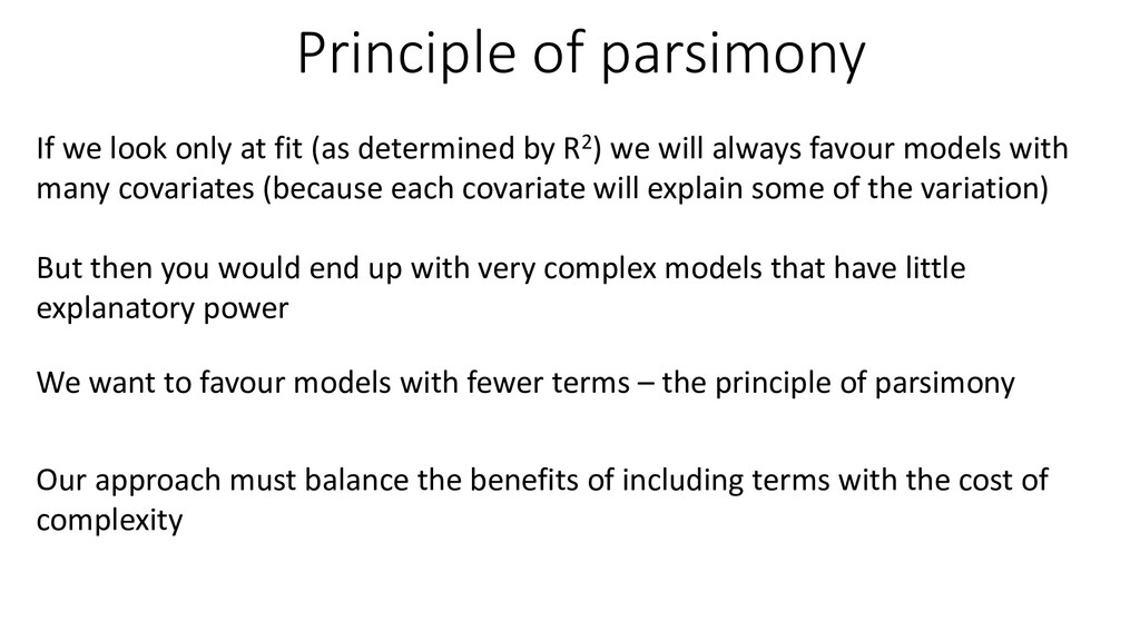
including terms with the cost of complexity If we look only at fit (as determined by R2) we will always favour models with many covariates (because each covariate will explain some of the variation) But then you would end up with very complex models that have little explanatory power We want to favour models with fewer terms – the principle of parsimony
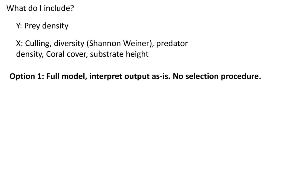
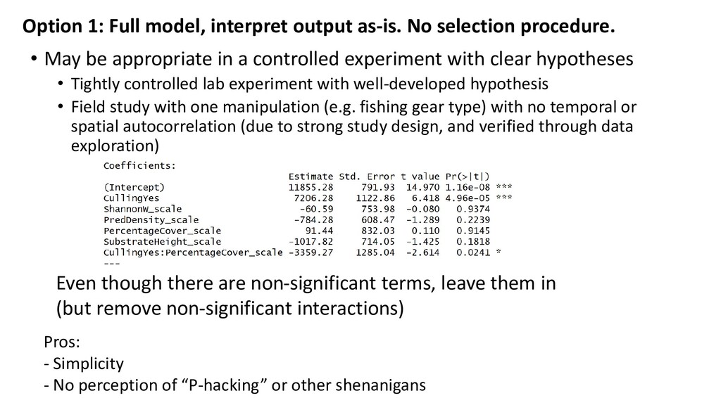
• May be appropriate in a controlled experiment with clear hypotheses • Tightly controlled lab experiment with well-developed hypothesis • Field study with one manipulation (e.g. fishing gear type) with no temporal or spatial autocorrelation (due to strong study design, and verified through data exploration) Even though there are non-significant terms, leave them in (but remove non-significant interactions) Pros: - Simplicity - No perception of “P-hacking” or other shenanigans
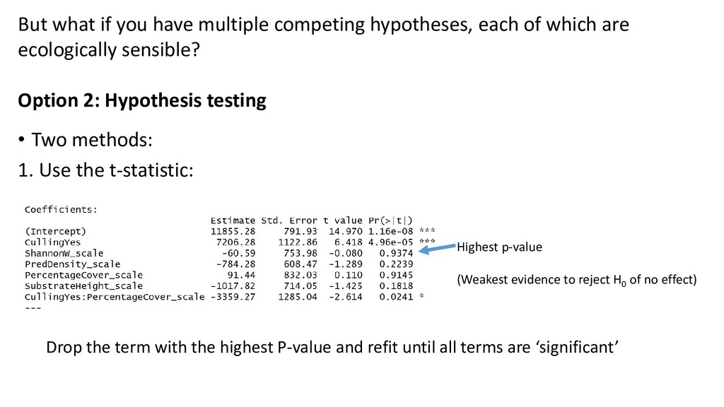
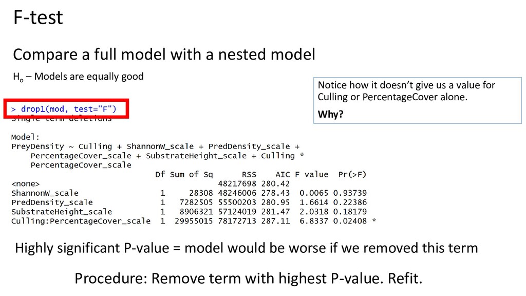
which are ecologically sensible? Option 2: Hypothesis testing • Two methods: 1. Use the t-statistic: Highest p-value (Weakest evidence to reject H0 of no effect) Drop the term with the highest P-value and refit until all terms are ‘significant’
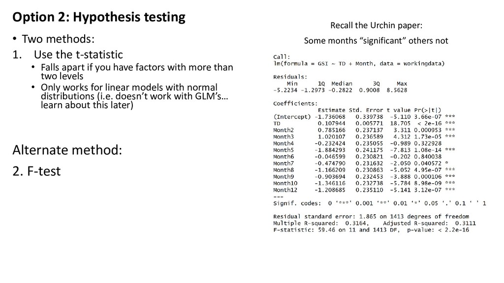
t-statistic • Falls apart if you have factors with more than two levels • Only works for linear models with normal distributions (i.e. doesn’t work with GLM’s… learn about this later) Recall the Urchin paper: Some months “significant” others not Alternate method: 2. F-test
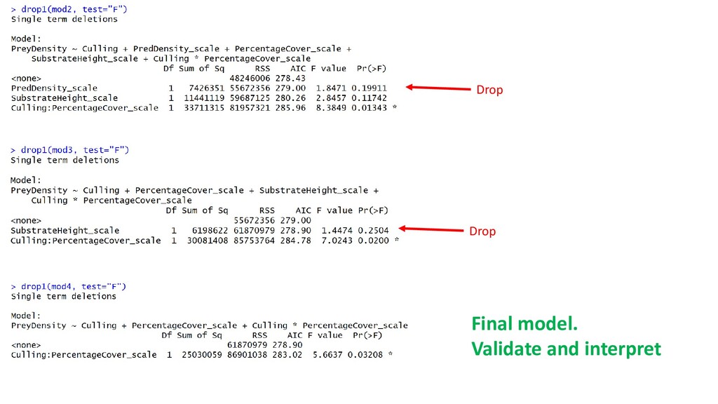
– Models are equally good Highly significant P-value = model would be worse if we removed this term Notice how it doesn’t give us a value for Culling or PercentageCover alone. Why? Procedure: Remove term with highest P-value. Refit.
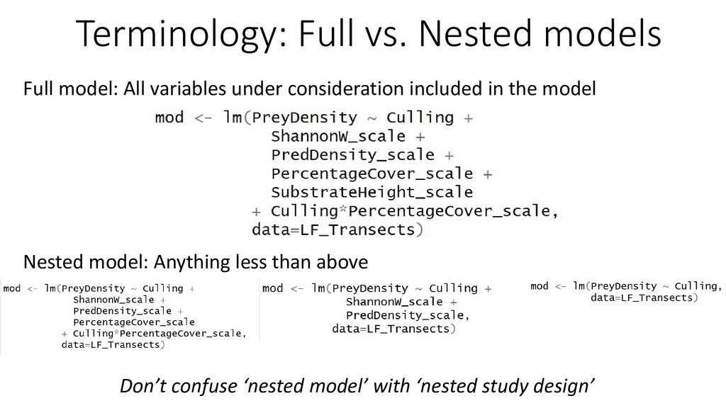
of steps – multiple comparisons problem. 5% chance of being wrong at each step! • If there is collinearity you missed, then stepping backwards could lead you on the wrong path • Only works with nested models Backwards selection – Start from full model and work backwards Forward selection – Start from reduced model, work towards full
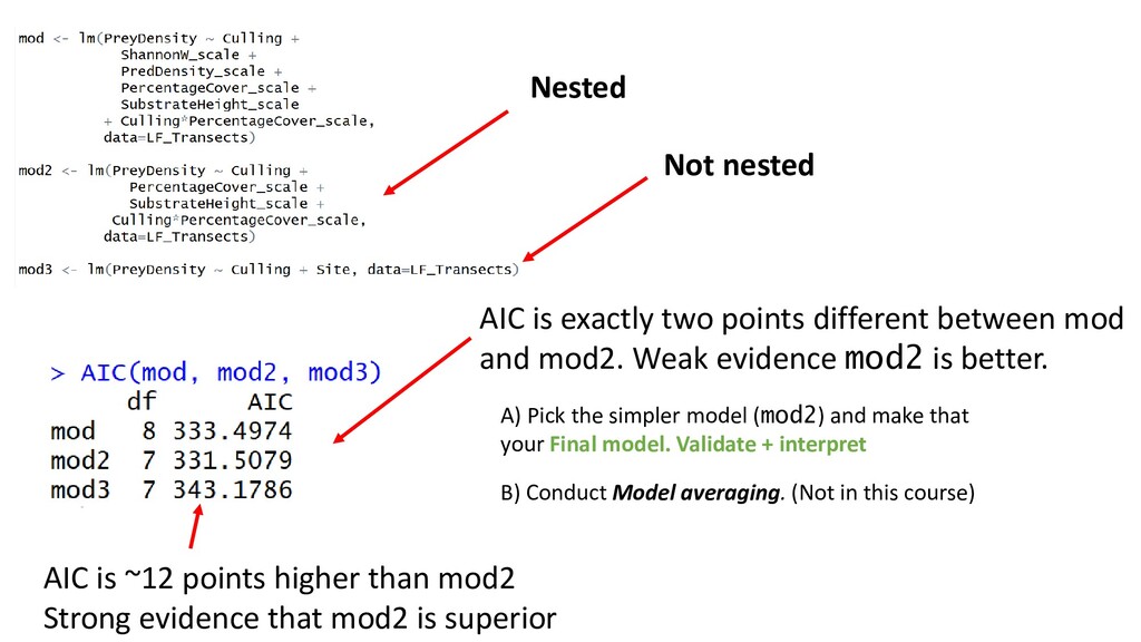
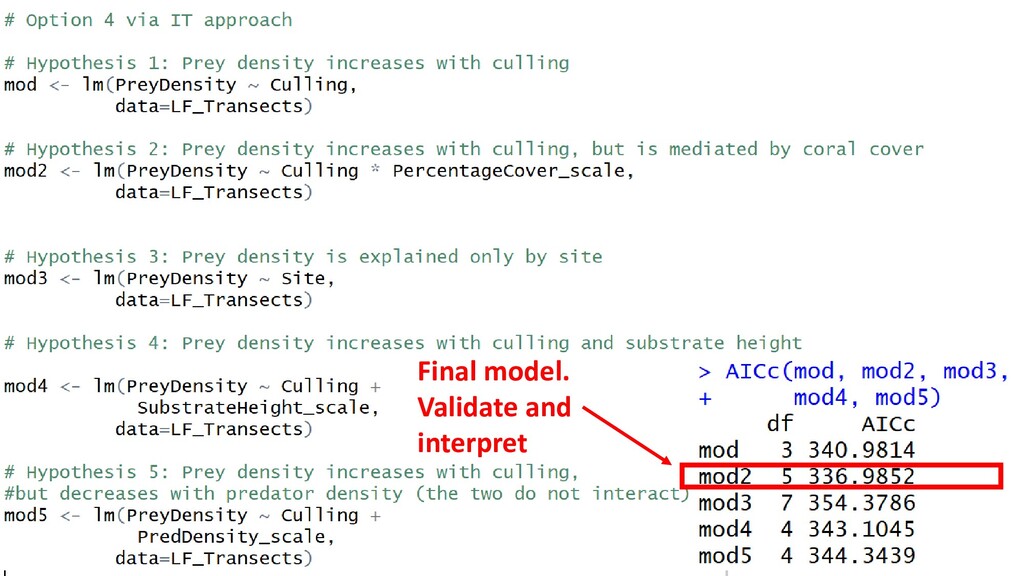
(AIC) Score: lower is better. Difference > 2 = meaningful Additional terms in the model increase AIC. Punishes complexity AIC meaningless on its own. It is solely for comparison Can be used with nested and non-nested models
Strong evidence that mod2 is superior AIC is exactly two points different between mod and mod2. Weak evidence mod2 is better. A) Pick the simpler model (mod2) and make that your Final model. Validate + interpret B) Conduct Model averaging. (Not in this course)
REMOVED this term If you removed the Interaction, AIC would be 285. If you remove Substrate Height AIC would be 280 (a better model) If you remove PredDensity, AIC would be 279 (equally good as removing Substrate Height)
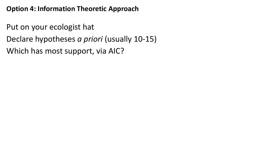
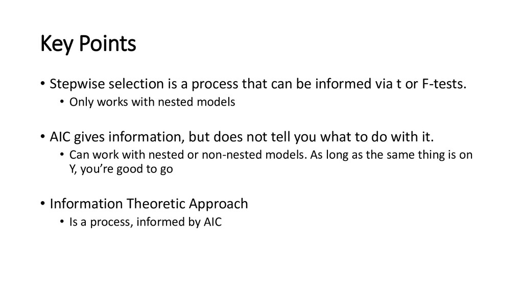
be informed via t or F-tests. • Only works with nested models • AIC gives information, but does not tell you what to do with it. • Can work with nested or non-nested models. As long as the same thing is on Y, you’re good to go • Information Theoretic Approach • Is a process, informed by AIC
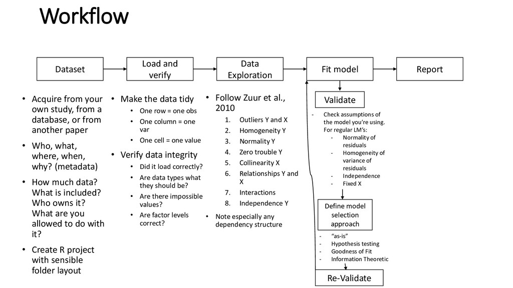
Define model selection approach Workflow • Acquire from your own study, from a database, or from another paper • Who, what, where, when, why? (metadata) • How much data? What is included? Who owns it? What are you allowed to do with it? • Create R project with sensible folder layout • Make the data tidy • One row = one obs • One column = one var • One cell = one value • Verify data integrity • Did it load correctly? • Are data types what they should be? • Are there impossible values? • Are factor levels correct? • Follow Zuur et al., 2010 1. Outliers Y and X 2. Homogeneity Y 3. Normality Y 4. Zero trouble Y 5. Collinearity X 6. Relationships Y and X 7. Interactions 8. Independence Y • Note especially any dependency structure - “as-is” - Hypothesis testing - Goodness of Fit - Information Theoretic - Check assumptions of the model you’re using. For regular LM’s: - Normality of residuals - Homogeneity of variance of residuals - Independence - Fixed X Re-Validate
• Note dependency structure, sample sizes per treatment, etc 3. Prep the data • Keep it tidy • Check all variables for typos, entry errors, impossible values • Note the types of data (counts, continuous measurement, yes/no, proportions, Likert, etc.) • Calculate derived quantities from raw data 4. Data exploration • Outliers Y and X • Homogeneity Y • Normality Y • Zeroes Y • Collinearity X • Relationships Y and X • Interactions • Independence Y 5. Present the statistical model • Write the equation and type of model • Cite a reference paper that explains the model, and the package you will use to run it • Decide whether to standardize covariates 6. Perform model selection • Or don’t. But own it. 7. Fit the final model 8. Validate the model • Check VIF, remove collinear covariates. Refit if necessary • Check assumptions. For linear models: • Normality • Homogeneity of variance • Independence • Fixed X Report model output in paper Show exploration and validation as an appendix Process may be interrupted by discoveries along the way (violations, etc) So far, you know how to: