How (Much) to Sample to Estimate the Mean

How (Much) to Sample to Estimate a Mean
Fred J. Hickernell
Illinois Institute of Technology
Dept. Applied Math Ctr. Interdisc. Scientific Comput. Office of Research
[email protected] sites.google.com/iit.edu/fred-j-hickernell
Thank you for your invitation and hospitality,
Slides at speakerdeck.com/fjhickernell/how-much-to-sample-to-estimate-the-mean
Jupyter notebook with figures at (H. 2023)
Purdue Statistics Colloquium, Friday, March 3, 2023

View Slide

Intro IID Low Discrepancy Software Summary References
Fred Is Like Dennis Lin
multicultural
multilingual
multicultural
multilingual
2/23

View Slide

Fred Is (Not) Like Dennis Lin
Colloquium Talk
multicultural
multilingual
multicultural
multilingual
2/23

View Slide

Computing the Mean, µ = E(Y)
Probability µ = y ϱ(y) dy, Y ∼ known ϱ
3/23

View Slide

Statistics µ ∈ ^
µ −
2.58^
σ
√
n
, ^
µ +
2.58^
σ
√
n
with high probability
^
µ =
1
n
n
i=1
Yi, ^
σ2 =
1
n − 1
n
i=1
(Yi − ^
µ)2,
Y1, Y2, . . . IID
∼ unknown ϱ
3/23

View Slide

Computer Experiments Y = f(X), X ∼ U[0, 1]d
µ =
[0,1]d
f(x) dx ∈ [^
µ − ε, ^
µ + ε], ε specified, fixed width
^
µ =
1
n
n
i=1
f(Xi), X1, X2, mimic
∼ U[0, 1]d
Statistics µ ∈ ^
µ −
2.58^
σ
√
n
, ^
µ +
2.58^
σ
√
n
with high probability
^
µ =
1
n
n
i=1
Yi, ^
σ2 =
1
n − 1
n
i=1
(Yi − ^
µ)2,
Y1, Y2, . . . IID
∼ unknown ϱ
3/23

View Slide

option payoff
flow velocity through rock with random porosity
Bayesian posterior density times parameter
µ =
[0,1]d
f(x) dx ∈ [^
µ − ε, ^
µ + ε], ε specified, fixed width
^
µ =
1
n
n
i=1
∼ U[0, 1]d
option price
mean flow velocity through rock with random porosity
Bayesian posterior mean
3/23

View Slide

µ =
[0,1]d
f(x) dx ∈ [^
µ − ε, ^
µ + ε], ε specified, fixed width, n
^
µ =
1
n
n
i=1
∼ U[0, 1]d
3/23

View Slide

Fixed-Width Central Limit Theorem (CLT) Confidence Intervals
Given random number generator Y1, Y2, . . . IID
∼ unknown ϱ
parameter nσ
Input error tolerance ε
Compute ^
µσ =
1
nσ
nσ
i=1
Yi, ^
σ2 =
1
nσ − 1
nσ
i=1
(Yi − ^
µσ)2
n =
2.58^
σ
ε
2
Output ^
µ =
1
n
nσ+n
i=nσ+1
Yi, µ ∈ [^
µ − ε, ^
µ + ε] with high probability
4/23

View Slide

Fixed-Width Central Limit Theorem (CLT) Confidence Intervals
Given random number generator Y1, Y2, . . . IID
∼ unknown ϱ
parameter nσ
Compute ^
µσ =
1
nσ
nσ
i=1
Yi, ^
σ2 =
1
nσ − 1
nσ
i=1
(Yi − ^
µσ)2
n =
2.58^
σ
ε
2
Output ^
µ =
1
n
nσ+n
i=nσ+1
Yi, µ ∈ [^
µ − ε, ^
µ + ε] with high probability
What might go wrong
Do not know how well ^
σ2 bounds var(Y)
CLT is an asymptotic (not finite sample) result
4/23

View Slide

Fixed-Width Confidence Intervals Assuming Bounded Kurtosis
Given Y1, Y2, . . . IID
∼ unknown ϱ, kurt(Y) ⩽ κmax
parameters nσ, κmax
Compute ^
µσ =
1
nσ
nσ
i=1
Yi, ^
σ2 =
1
nσ − 1
nσ
i=1
(Yi − ^
µσ)2,
n = CBE
Cσ(κmax
, nσ)^
σ
ε
, κmax
Output ^
µ =
1
n
nσ+n
i=nσ+1
Yi, µ ∈ [^
µ − ε, ^
µ + ε] with 99% probability
The fix (H., Jiang, Liu, and Owen 2013)
var(Y) ⩽ C2
σ
(κmax
, nσ)^
σ2 with probability
√
99%
Berry-Esseen inequality gives finite sample
√
99% confidence interval
5/23

View Slide

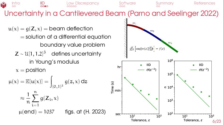
Uncertainty in a Cantilevered Beam (Parno and Seelinger 2022)
u(x) = g(Z, x) = beam deflection
= solution of a differential equation
boundary value problem
Z ∼ U[1, 1.2]3 defines uncertainty
in Young’s modulus
x = position
µ(x) = E[u(x)] =
[0,1]3
g(z, x) dz
≈
1
n
n
i=1
g(Zi, x)
µ(end) = 1037 figs. at (H. 2023)
101 102
Tolerance, ε
sec
min
hr
Time (s)
IID
(ε−2)
101 102
Tolerance, ε
102
103
104
105
106
n
IID
(ε−2)
6/23

View Slide

Cones Are Better than Balls for Adaptive Algorithms
Fixed Width Confidence Intervals (using IID sampling)
Y = Y : E[(Y − µ)4]
var2(Y)
⩽ κmax
Y = Y : var(Y) ⩽ σ2
max
Use Berry-Esseen inequality Use Chebyshev inequality
Y is not too heavy tailed Y is not too big
Y ∈ Y =⇒ aY ∈ Y Y ∈ Y ̸
=⇒ aY ∈ Y
Adaptive sample size Fixed sample size
7/23

View Slide

Cones Are Better than Balls for Adaptive Algorithms
Fixed Width Confidence Intervals (using IID sampling)
Y = Y : E[(Y − µ)4]
var2(Y)
⩽ κmax
Y = Y : var(Y) ⩽ σ2
max
Use Berry-Esseen inequality Use Chebyshev inequality
Y is not too heavy tailed Y is not too big
Y ∈ Y =⇒ aY ∈ Y Y ∈ Y ̸
=⇒ aY ∈ Y
Adaptive sample size Fixed sample size
Choice of inflation factors
depends on or implies κmax
Non-convex cones may permit successful adaptive algorithms
(Bahadur and Savage 1956; Bakhvalov 1970)
7/23

View Slide

Low Discrepancy Samples Fill Space Better
0 1
xi,1
0
1
xi,2
n = 64
0 1
xi,1
0
1
xi,2
n = 128
0 1
xi,1
0
1
xi,2
n = 256
0 1
xi,1
0
1
xi,2
n = 512
IID Points
0 1
xi, 1
0
1
xi, 2
n = 64
0 1
xi, 1
0
1
xi, 2
n = 128
0 1
xi, 1
0
1
xi, 2
n = 256
0 1
xi, 1
0
1
xi, 2
n = 512
Lattice Points
8/23

View Slide

Low Discrepancy Samples Fill Space Better
0 1
xi,1
0
1
xi,2
n = 64
0 1
xi,1
0
1
xi,2
n = 128
0 1
xi,1
0
1
xi,2
n = 256
0 1
xi,1
0
1
xi,2
n = 512
IID Points
0 1
xi, 1
0
1
xi, 2
n = 64
0 1
xi, 1
0
1
xi, 2
n = 128
0 1
xi, 1
0
1
xi, 2
n = 256
0 1
xi, 1
0
1
xi, 2
n = 512
Sobol' Points
8/23

View Slide

Low Discrepancy Samples Approximate Integrals Better
Discrepancy measures how far the empirical distribution of {x1, . . . , xn} is from the
uniform distribution (H. 1999; Niederreiter 1992)
µ
[0,1]d
f(x) dx −
1
n
n
i=1
f(xi) ⩽
sample quality
discrepancy(x1, . . . , xn) ×
function roughness
semi-norm(f)
0 1
xi, 1
0
1
xi, 2
n = 64
0 1
xi, 1
0
1
xi, 2
n = 128
0 1
xi, 1
0
1
xi, 2
n = 256
0 1
xi, 1
0
1
xi, 2
n = 512
Lattice Points
9/23

View Slide

Low Discrepancy Samples Approximate Integrals Better
Discrepancy measures how far the empirical distribution of {x1, . . . , xn} is from the
uniform distribution (H. 1999; Niederreiter 1992)
µ
[0,1]d
f(x) dx −
1
n
n
i=1
f(xi) ⩽
sample quality
discrepancy(x1, . . . , xn)
expensive to compute
×
function roughness
semi-norm(f)
no way to bound
0 1
xi, 1
0
1
xi, 2
n = 64
0 1
xi, 1
0
1
xi, 2
n = 128
0 1
xi, 1
0
1
xi, 2
n = 256
0 1
xi, 1
0
1
xi, 2
n = 512
Lattice Points
9/23

View Slide

Fixed-Width Confidence Intervals via Lattice Sampling
f(x) =
k∈Zd
f(k) exp(2π
√
−1k′x), f(k) =
[0,1]d
f(x) exp(−2π
√
−1k′x) dx Fourier series
µ
[0,1]d
f(x) dx
f(0)
−
1
n
n
i=1
f(xi) =
k∈Zd
k′xi∈Z ∀i
f(k)
⩽
k∈Zd
k′xi∈Z ∀i
f(k) depends on terms aliased w/ constant
⩽
k∈Zd
k′xi∈Z ∀i
1
|weight(k)|2
discrepancy(x1,...,xn)
×
0̸=k∈Zd
f(k)weight(k) 2
semi-norm(f)
10/23

View Slide

Fixed-Width Confidence Intervals via Lattice Sampling
f(x) =
k∈Zd
f(k) exp(2π
√
−1k′x), f(k) =
[0,1]d
f(x) exp(−2π
√
−1k′x) dx Fourier series
µ
[0,1]d
f(x) dx
f(0)
−
1
n
n
i=1
f(xi) ⩽
k∈Zd
k′xi∈Z ∀i
f(k) depends on terms aliased w/ constant
Adaptive stopping rule for lattices (H. and Jiménez Rugama 2016)
Define = {f whose Fourier coefficients decay nicely}
Bound
k∈Zd
k′xi∈Z ∀i
f(k) in terms of sums of f(k) =
1
n
n
i=1
f(xi) exp(−2π
√
−1k′x)
fast Fourier transform
for f ∈
Increase n until error bound ⩽ ε 10/23

View Slide

IID vs. Low Discrepancy for the Cantilevered Beam
x = position
µ(x) = E[u(x)] ≈ 1037
10−2 10−1 100 101 102
Tolerance, ε
sec
min
hr
Time (s)
Lattice
(ε−1)
IID
(ε−2)
10−2 10−1 100 101 102
Tolerance, ε
102
103
104
105
106
n
Lattice
(ε−1)
IID
(ε−2)
11/23

View Slide

There Is More
Adaptive stopping criteria also available for
▶ Sobol’ points (Jiménez Rugama and H. 2016), but not Halton
▶ Relative and hybrid error criteria (H., Jiménez Rugama, and Li 2018)
▶ Multiple answers based on a number of integrals, such as Sobol’ indices (Sorokin
and Jagadeeswaran 2022+)
12/23

View Slide

There Is More
Adaptive stopping criteria also available for
▶ Sobol’ points (Jiménez Rugama and H. 2016), but not Halton
▶ Relative and hybrid error criteria (H., Jiménez Rugama, and Li 2018)
▶ Multiple answers based on a number of integrals, such as Sobol’ indices (Sorokin
and Jagadeeswaran 2022+)
Bayesian adaptive stopping criteria (Jagadeeswaran and H. 2019, 2022)
where
▶ f is an instance of a Gaussian process
▶ Credible interval gives the error bound
▶ Covariance kernel has hyperparameters that are tuned by empirical Bayes or
cross-validation
▶ Choosing kernels that partner with lattice or Sobol’ makes computation efficient
(O(n log n) not O(n3))
12/23

View Slide

Where to Find Low Discrepancy Sequences
BRODA (Kucherenko 2022)
Dakota (Adams, Bohnhoff, et al. 2022)
Julia (SciML QuasiMonteCarlo.jl 2022)
MATLAB (The MathWorks, Inc. 2022)
NAG (The Numerical Algorithms Group 2021)
PyTorch (Paszke, Gross, et al. 2019)
R (Hofert and Lemieux 2017)
SAS (SAS Institute 2023)
SciPy (Virtanen, Gommers, et al. 2020)
TensorFlow (TF Quant Finance Contributors 2021),
but beware of some limited, outdated, and incorrect implementations
13/23

View Slide

QMCPy, a Python quasi-Monte Carlo Library
Quasi-Monte Carlo methods use low discrepancy sampling
Open source project (Choi, H., et al. 2022)
A blog qmcpy.org
Low discrepancy generators
Variable transformations
Stopping criteria
Links with models via UM-Bridge (Davis, Parno, Reinarz, and Seelinger 2022)
14/23

View Slide

The Whole Cantilevered Beam
x = position
0 10 20 30
x
0
250
500
750
1000
u(x)
Cantilevered Beam
10−2 10−1 100
Tolerance, ε
sec
min
Time (s)
Lattice
(ε−1)
Lattice Parallel
(ε−1)
10−2 10−1 100
Tolerance, ε
101
102
103
104
105
106
n
Lattice
(ε−1)
Lattice Parallel
(ε−1)
15/23

View Slide

Take Aways
How to sample?
▶ Low discrepancy sequences (aka quasi-Monte Carlo methods) for high efficiency
How much to sample?
▶ Data-based, theoretically justified adaptive stopping criteria
Traditional theory impractical
Based on cones of random variables or integrands
16/23

View Slide

Take Aways
How to sample?
▶ Better variable transforms needed for peaky f
How much to sample?
▶ Criteria and theory needed for
Multilevel methods
Densities and quantiles
16/23

View Slide

Take Aways
How to sample?
▶ Better variable transforms needed for peaky f
How much to sample?
▶ Criteria and theory needed for
Multilevel methods
Densities and quantiles
Use and develop good software, make research reproducible (H. 2023)
16/23

View Slide

Thank you
These slides are available at
speakerdeck.com/fjhickernell/how-much-to-sample-to-estimate-the-mean
Jupyter notebook with figures at (H. 2023)

View Slide

References I
H., F. J. (1999). “Goodness-of-Fit Statistics, Discrepancies and Robust Designs”.
In: Statist. Probab. Lett. 44, pp. 73–78. doi: 10.1016/S0167-7152(98)00293-4.
— (2023). Jupyter Notebook for Computations and Figures for the 2023 March
3 Statistics Colloquium at Purdue University. https://github.com/QMCSoftware/
QMCSoftware/blob/Purdue2023Talk/demos/Purdue_Talk_Figures.ipynb.
H., F. J. and Ll. A. Jiménez Rugama (2016). “Reliable Adaptive Cubature Using
Digital Sequences”. In: Monte Carlo and Quasi-Monte Carlo Methods:
MCQMC, Leuven, Belgium, April 2014. Ed. by R. Cools and D. Nuyens. Vol. 163.
Springer Proceedings in Mathematics and Statistics. arXiv:1410.8615 [math.NA].
Springer-Verlag, Berlin, pp. 367–383.
18/23

View Slide

References II
H., F. J., Ll. A. Jiménez Rugama, and D. Li (2018). “Adaptive Quasi-Monte Carlo
Methods for Cubature”. In: Contemporary Computational Mathematics — a
celebration of the 80th birthday of Ian Sloan. Ed. by J. Dick, F. Y. Kuo, and
H. Woźniakowski. Springer-Verlag, pp. 597–619. doi: 10.1007/978-3-319-72456-0.
H., F. J. et al. (2013). “Guaranteed Conservative Fixed Width Confidence
Intervals Via Monte Carlo Sampling”. In: Monte Carlo and Quasi-Monte Carlo
Methods 2012. Ed. by J. Dick et al. Vol. 65. Springer Proceedings in Mathematics
and Statistics. Springer-Verlag, Berlin, pp. 105–128. doi:
10.1007/978-3-642-41095-6.
Adams, Brian M. et al. (May 2022). Dakota, A Multilevel Parallel
Object-Oriented Framework for Design Optimization, Parameter Estimation,
Uncertainty Quantification, and Sensitivity Analysis: Version 6.16 User’s Manual.
Sandia National Laboratories.
19/23

View Slide

References III
Bahadur, R. R. and L. J. Savage (1956). “The Nonexistence of Certain Statistical
Procedures in Nonparametric Problems”. In: Ann. Math. Stat. 27, pp. 1115–1122.
Bakhvalov, N. S. (1970). “On the optimality of linear methods for operator
approximation in convex classes of functions (in Russian)”. In: Zh. Vychisl. Mat. i
Mat. Fiz. 10. English transl.: USSR Comput. Math. Math. Phys. 11 (1971) 244–249.,
pp. 555–568.
Choi, S.-C. T. et al. (2022). QMCPy: A quasi-Monte Carlo Python Library. doi:
10.5281/zenodo.3964489. url: https://qmcsoftware.github.io/QMCSoftware/.
Cools, R. and D. Nuyens, eds. (2016). Monte Carlo and Quasi-Monte Carlo
Methods: MCQMC, Leuven, Belgium, April 2014. Vol. 163. Springer Proceedings
in Mathematics and Statistics. Springer-Verlag, Berlin.
Davis, A. et al. (2022). UQ and Model Bridge (UM-Bridge). url:
https://um-bridge-benchmarks.readthedocs.io/en/docs/.
20/23

View Slide

References IV
Hofert, M. and C. Lemieux (2017). qrng R package. url:
https://cran.r-project.org/web/packages/qrng/qrng.pdf (visited on 2017).
Jagadeeswaran, R. and F. J. H. (2019). “Fast Automatic Bayesian Cubature
Using Lattice Sampling”. In: Stat. Comput. 29, pp. 1215–1229. doi:
10.1007/s11222-019-09895-9.
— (2022). “Fast Automatic Bayesian Cubature Using Sobol’ Sampling”. In:
Advances in Modeling and Simulation: Festschrift in Honour of Pierre L’Ecuyer.
Ed. by Z. Botev et al. Springer, Cham, pp. 301–318. doi:
10.1007/978-3-031-10193-9\_15.
Jiménez Rugama, Ll. A. and F. J. H. (2016). “Adaptive Multidimensional
Integration Based on Rank-1 Lattices”. In: Monte Carlo and Quasi-Monte Carlo
Methods: MCQMC, Leuven, Belgium, April 2014. Ed. by R. Cools and D. Nuyens.
Vol. 163. Springer Proceedings in Mathematics and Statistics. arXiv:1411.1966.
Springer-Verlag, Berlin, pp. 407–422.
21/23

View Slide

References V
Kucherenko, S. (2022). BRODA. url: https://www.broda.co.uk/index.html.
Niederreiter, H. (1992). Random Number Generation and Quasi-Monte Carlo
Methods. CBMS-NSF Regional Conference Series in Applied Mathematics.
Philadelphia: SIAM.
Parno, M. and L. Seelinger (2022). Uncertainty propagation of material
properties of a cantilevered beam. url:
https://um-bridge-benchmarks.readthedocs.io/en/docs/forward-
benchmarks/muq-beam-propagation.html.
Paszke, Adam et al. (2019). “PyTorch: An imperative style, high-performance
deep learning library”. In: Advances in neural information processing systems
32, pp. 8026–8037.
SAS Institute (2023). SAS Documentation for the MODEL Procedure. url:
https://documentation.sas.com/doc/en/pgmsascdc/9.4_3.4/etsug/etsug_model_
sect197.htm.
22/23

View Slide

References VI
SciML QuasiMonteCarlo.jl (2022). url:
https://github.com/SciML/QuasiMonteCarlo.jl.
Sorokin, A. G. and R. Jagadeeswaran (2022+). “Monte Carlo for Vector
Functions of Integrals”. In: Monte Carlo and Quasi-Monte Carlo Methods:
MCQMC, Linz, Austria, July 2022. Ed. by A. Hinrichs, P. Kritzer, and
F. Pillichshammer. Springer Proceedings in Mathematics and Statistics. in
preparation for submission for publication. Springer, Cham.
TF Quant Finance Contributors (2021). Quasi Monte-Carlo Methods. url:
https://github.com/google/tf-quant-finance/math/qmc.
The MathWorks, Inc. (2022). MATLAB R2022b. Natick, MA.
The Numerical Algorithms Group (2021). The NAG Library. Mark 27. Oxford.
Virtanen, Pauli et al. (2020). “SciPy 1.0: fundamental algorithms for scientific
computing in Python”. In: Nature Methods 17.3, pp. 261–272.
23/23

View Slide

How (Much) to Sample to Estimate the Mean

How (Much) to Sample to Estimate the Mean

Fred J. Hickernell

More Decks by Fred J. Hickernell

Other Decks in Research

Featured

Transcript