Measures of Error, Discrepancy, and Complexity

Talk to SAMSI-QMC WG-V on October 18, 2017

Transcript

1. Measures of Error, Discrepancy, and Complexity Fred J. Hickernell Department of Applied Mathematics, Illinois Institute of Technology hickernell@iit.edu mypages.iit.edu/~hickernell Thanks to the Guaranteed Automatic Integration Library (GAIL) team and friends Supported by NSF-DMS-1522687 Working Group V, Ocotober 18, 2017
2. Problem One-Dimensional Problems Multiple Dimensions References Problem Given an error tolerance, ε, and a black-box, f, that accepts inputs, x ∈ Ω and produces outputs, f(x) ∈ R, Carefully choose the number and positions of inputs, {xi}n i=1 ⊂ Ω, and then use the output data, {f(xi)}n i=1 , to construct an approximate solution, app {(xi, f(xi))}n i=1 , ε sol(f) = Ω f(x) dx or f(x) app {(xi, f(xi))}n i=1 , ε = n i=1 wif(xi) or n i=1 wi(x)f(xi) satisfying sol(f) − app {(xi, f(xi))}n i=1 , ε errn({xi}n i=1 , f) ε We focus on linear problems. For fixed {xi}n i=1 , app {(xi, f(xi))}n i=1 , ε is linear, but the choices of n, and the xi, may depend nonlinearly on f. 2/17
3. Problem One-Dimensional Problems Multiple Dimensions References (One-Dimensional) Quadrature by Simple Average Suppose the functions belong to a Hilbert space H = f : Ω = [−1, 1] → R f 2 < ∞ with f, g H = f(0)g(0) + 1 2 1 −1 f (x)g (x) dx 3/17
4. Problem One-Dimensional Problems Multiple Dimensions References (One-Dimensional) Quadrature by Simple Average Suppose the functions belong to a Hilbert space H = f : Ω = [−1, 1] → R f 2 < ∞ with f, g H = f(0)g(0) + 1 2 1 −1 f (x)g (x) dx The reproducing kernel K : [−1, 1] × [−1, 1] → R is defined by K(x, t) = 1 + |x| + |t| − |x − t| N. Aronszajn. Theory of Reproducing Kernels. Trans. Amer. Math. Soc. 68, 337–404 (1950), H., F. J. A Generalized Discrepancy and Quadrature Error Bound. Math. Comp. 67, 299–322 (1998). 3/17
5. Problem One-Dimensional Problems Multiple Dimensions References (One-Dimensional) Quadrature by Simple Average Suppose the functions belong to a Hilbert space H = f : Ω = [−1, 1] → R f 2 < ∞ with f, g H = f(0)g(0) + 1 2 1 −1 f (x)g (x) dx The reproducing kernel K : [−1, 1] × [−1, 1] → R is defined by K(x, t) = 1 + |x| + |t| − |x − t| To verify, note that K(x, t) = K(t, x) ∀x, t ∈ [−1, 1] K(·, t) ∈ H ∀t since K(·, t) 2 H = |K(0, t)|2 + 1 2 1 −1 ∂K ∂x (x, t) 2 dx = 1 − 2 |t| < ∞ K(·, t), f H = 1 × f(0) + 1 2 1 −1 [sign(x) − sign(x − t)] f (x) dx = f(t) ∀t ∈ [−1, 1] N. Aronszajn. Theory of Reproducing Kernels. Trans. Amer. Math. Soc. 68, 337–404 (1950), H., F. J. A Generalized Discrepancy and Quadrature Error Bound. Math. Comp. 67, 299–322 (1998). 3/17
6. Problem One-Dimensional Problems Multiple Dimensions References (One-Dimensional) Quadrature by Simple Average cont’d f, g H = f(0)g(0)+ 1 2 1 −1 f (x)g (x) dx, K(x, t) = 1+|x|+|t|−|x − t| , K(·, t), f H = f(t) Let sol(f) = 1 −1 f(x) dx and quadn (f) = 2 n n i=1 f 2i − n − 1 n . Then by the Riesz representation theorem and the Cauchy-Schwartz inequality sol(f) − quadn (f) = ηn, f H , |sol(f) − quadn (f)| ηn H f H , 4/17
7. Problem One-Dimensional Problems Multiple Dimensions References (One-Dimensional) Quadrature by Simple Average cont’d f, g H = f(0)g(0)+ 1 2 1 −1 f (x)g (x) dx, K(x, t) = 1+|x|+|t|−|x − t| , K(·, t), f H = f(t) Let sol(f) = 1 −1 f(x) dx and quadn (f) = 2 n n i=1 f 2i − n − 1 n . Then by the Riesz representation theorem and the Cauchy-Schwartz inequality sol(f) − quadn (f) = ηn, f H , |sol(f) − quadn (f)| ηn H f H , and by the reproducing property, ηn(t) = K(·, t), ηn H = sol(K(·, t)) − quadn (K(·, t)), and ηn 2 H = ηn, ηn H = sol(ηn) − quadn (ηn) = sol·· sol·(K(·, ··) − 2 sol·· quad· n (K(·, ··) + quad·· n quad· n (K(·, ··) = 16 3 − 4 n n i=1 2 + 2 2i − n − 1 n − 2i − 1 2n 2 + 4 n2 n i,k=1 1 + 2i − n − 1 n + 2k − n − 1 n − 2i − 2k n 4/17
8. Problem One-Dimensional Problems Multiple Dimensions References (One-Dimensional) Quadrature by Simple Average cont’d f, g H = f(0)g(0)+ 1 2 1 −1 f (x)g (x) dx, K(x, t) = 1+|x|+|t|−|x − t| , K(·, t), f H = f(t) Let sol(f) = 1 −1 f(x) dx and quadn (f) = 2 n n i=1 f 2i − n − 1 n . Then by the Riesz representation theorem and the Cauchy-Schwartz inequality sol(f) − quadn (f) = ηn, f H , |sol(f) − quadn (f)| ηn H f H , and by the reproducing property, ηn(t) = K(·, t), ηn H = sol(K(·, t)) − quadn (K(·, t)), and ηn 2 H = ηn, ηn H = sol(ηn) − quadn (ηn) = sol·· sol·(K(·, ··) − 2 sol·· quad· n (K(·, ··) + quad·· n quad· n (K(·, ··) = 16 3 − 4 n n i=1 2 + 2 2i − n − 1 n − 2i − 1 2n 2 + 4 n2 n i,k=1 1 + 2i − n − 1 n + 2k − n − 1 n − 2i − 2k n = 4 3n2 4/17
9. Problem One-Dimensional Problems Multiple Dimensions References (One-Dimensional) Quadrature by Simple Average cont’d f, g H = f(0)g(0)+ 1 2 1 −1 f (x)g (x) dx, K(x, t) = 1+|x|+|t|−|x − t| , K(·, t), f H = f(t) Let sol(f) = 1 −1 f(x) dx and quadn (f) = 2 n n i=1 f 2i − n − 1 n . Then by the Riesz representation theorem and the Cauchy-Schwartz inequality sol(f) − quadn (f) = ηn, f H , |sol(f) − quadn (f)| ηn H f H , and by the reproducing property, ηn(t) = K(·, t), ηn H = sol(K(·, t)) − quadn (K(·, t)) 4/17
10. Problem One-Dimensional Problems Multiple Dimensions References (One-Dimensional) Quadrature by Simple Average cont’d f, g H = f(0)g(0) + 1 2 1 −1 f (x)g (x) dx, K(x, t) = 1 + |x| + |t| − |x − t| , K(·, t), f H = f(t) sol(f) = 1 −1 f(x) dx, quadn (f) = 2 n n i=1 f 2i − n − 1 n , |sol(f) − quadn (f)| ηn H f H = 2 √ 3n [f(0)]2 + 1 2 1 −1 [f (x)]2 dx ηn H is called the discrepancy, it also has a geometric interpretation H., F. J. What Affects the Accuracy of Quasi-Monte Carlo Quadrature?. in Monte Carlo and Quasi-Monte Carlo Methods 1998 (eds Niederreiter, H. & Spanier, J.) (Springer-Verlag, Berlin, 2000), 16–55. 5/17
11. Problem One-Dimensional Problems Multiple Dimensions References (One-Dimensional) Quadrature by Simple Average cont’d f, g H = f(0)g(0) + 1 2 1 −1 f (x)g (x) dx, K(x, t) = 1 + |x| + |t| − |x − t| , K(·, t), f H = f(t) sol(f) = 1 −1 f(x) dx, quadn (f) = 2 n n i=1 f 2i − n − 1 n , |sol(f) − quadn (f)| ηn H f H = 2 √ 3n [f(0)]2 + 1 2 1 −1 [f (x)]2 dx ηn H is called the discrepancy, it also has a geometric interpretation H., F. J. What Affects the Accuracy of Quasi-Monte Carlo Quadrature?. in Monte Carlo and Quasi-Monte Carlo Methods 1998 (eds Niederreiter, H. & Spanier, J.) (Springer-Verlag, Berlin, 2000), 16–55. 6/17
12. Problem One-Dimensional Problems Multiple Dimensions References (One-Dimensional) Quadrature by Simple Average cont’d f, g H = f(0)g(0) + 1 2 1 −1 f (x)g (x) dx, K(x, t) = 1 + |x| + |t| − |x − t| , K(·, t), f H = f(t) sol(f) = 1 −1 f(x) dx, quadn (f) = 2 n n i=1 f 2i − n − 1 n , |sol(f) − quadn (f)| ηn H f H = 2 √ 3n [f(0)]2 + 1 2 1 −1 [f (x)]2 dx ηn H is called the discrepancy, it also has a geometric interpretation Why doesn’t the midpoint rule have faster decay? 6/17
13. Problem One-Dimensional Problems Multiple Dimensions References (One-Dimensional) Quadrature by Simple Average cont’d f, g H = f(0)g(0) + 1 2 1 −1 f (x)g (x) dx, K(x, t) = 1 + |x| + |t| − |x − t| , K(·, t), f H = f(t) sol(f) = 1 −1 f(x) dx, quadn (f) = 2 n n i=1 f 2i − n − 1 n , |sol(f) − quadn (f)| ηn H f H = 2 √ 3n [f(0)]2 + 1 2 1 −1 [f (x)]2 dx ηn H is called the discrepancy, it also has a geometric interpretation Why doesn’t the midpoint rule have faster decay? H is not smooth enough 6/17
14. Problem One-Dimensional Problems Multiple Dimensions References (One-Dimensional) Quadrature by Simple Average cont’d f, g H = f(0)g(0) + 1 2 1 −1 f (x)g (x) dx, K(x, t) = 1 + |x| + |t| − |x − t| , K(·, t), f H = f(t) sol(f) = 1 −1 f(x) dx, quadn (f) = 2 n n i=1 f 2i − n − 1 n , |sol(f) − quadn (f)| ηn H f H = 2 √ 3n [f(0)]2 + 1 2 1 −1 [f (x)]2 dx ηn H is called the discrepancy, it also has a geometric interpretation Why doesn’t the midpoint rule have faster decay? H is not smooth enough Can we extend this to arbitrary data sites, quadn (f) = 2 n n i=1 f(xi)? 6/17
15. Problem One-Dimensional Problems Multiple Dimensions References (One-Dimensional) Quadrature by Simple Average cont’d f, g H = f(0)g(0) + 1 2 1 −1 f (x)g (x) dx, K(x, t) = 1 + |x| + |t| − |x − t| , K(·, t), f H = f(t) sol(f) = 1 −1 f(x) dx, quadn (f) = 2 n n i=1 f 2i − n − 1 n , |sol(f) − quadn (f)| ηn H f H = 2 √ 3n [f(0)]2 + 1 2 1 −1 [f (x)]2 dx ηn H is called the discrepancy, it also has a geometric interpretation Why doesn’t the midpoint rule have faster decay? H is not smooth enough Can we extend this to arbitrary data sites, quadn (f) = 2 n n i=1 f(xi)? Yes ηn 2 H = 16 3 − 4 n n i=1 2 + 2 |xi| − |xi|2 + 4 n2 n i,k=1 [1 + |xi| + |xk | − |xi − xk |] 6/17
16. Problem One-Dimensional Problems Multiple Dimensions References (One-Dimensional) Quadrature by Simple Average cont’d f, g H = f(0)g(0) + 1 2 1 −1 f (x)g (x) dx, K(x, t) = 1 + |x| + |t| − |x − t| , K(·, t), f H = f(t) sol(f) = 1 −1 f(x) dx, quadn (f) = 2 n n i=1 f 2i − n − 1 n , |sol(f) − quadn (f)| ηn H f H = 2 √ 3n [f(0)]2 + 1 2 1 −1 [f (x)]2 dx ηn H is called the discrepancy, it also has a geometric interpretation Can we extend this to arbitrary weights, quadn (f) = n i=1 wif(xi)? 6/17
17. Problem One-Dimensional Problems Multiple Dimensions References (One-Dimensional) Quadrature by Simple Average cont’d f, g H = f(0)g(0) + 1 2 1 −1 f (x)g (x) dx, K(x, t) = 1 + |x| + |t| − |x − t| , K(·, t), f H = f(t) sol(f) = 1 −1 f(x) dx, quadn (f) = 2 n n i=1 f 2i − n − 1 n , |sol(f) − quadn (f)| ηn H f H = 2 √ 3n [f(0)]2 + 1 2 1 −1 [f (x)]2 dx ηn H is called the discrepancy, it also has a geometric interpretation Can we extend this to arbitrary weights, quadn (f) = n i=1 wif(xi)? Yes ηn 2 H = 16 3 − 2 n i=1 wi 2 + 2 |xi| − |xi|2 + n i,k=1 wiwk [1 + |xi| + |xk | − |xi − xk |] 6/17
18. Problem One-Dimensional Problems Multiple Dimensions References (One-Dimensional) Quadrature by Simple Average cont’d f, g H = f(0)g(0) + 1 2 1 −1 f (x)g (x) dx, K(x, t) = 1 + |x| + |t| − |x − t| , K(·, t), f H = f(t) sol(f) = 1 −1 f(x) dx, quadn (f) = 2 n n i=1 f 2i − n − 1 n , |sol(f) − quadn (f)| ηn H f H = 2 √ 3n [f(0)]2 + 1 2 1 −1 [f (x)]2 dx ηn H is called the discrepancy, it also has a geometric interpretation Can we extend this to arbitrary weights, quadn (f) = n i=1 wif(xi)? Yes How do we choose n to make |sol(f) − quadn (f)| ε? 6/17
19. Problem One-Dimensional Problems Multiple Dimensions References (One-Dimensional) Quadrature by Simple Average cont’d f, g H = f(0)g(0) + 1 2 1 −1 f (x)g (x) dx, K(x, t) = 1 + |x| + |t| − |x − t| , K(·, t), f H = f(t) sol(f) = 1 −1 f(x) dx, quadn (f) = 2 n n i=1 f 2i − n − 1 n , |sol(f) − quadn (f)| ηn H f H = 2 √ 3n [f(0)]2 + 1 2 1 −1 [f (x)]2 dx ηn H is called the discrepancy, it also has a geometric interpretation Can we extend this to arbitrary weights, quadn (f) = n i=1 wif(xi)? Yes How do we choose n to make |sol(f) − quadn (f)| ε? If f ∈ BR = {f : f H R}, then choose n such that ηn H ε/R. For the midpoint rule n √ 3R/(2ε). Not easy, since f H is unknown. 6/17
20. Problem One-Dimensional Problems Multiple Dimensions References (One-Dimensional) Quadrature by Simple Average cont’d f, g H = f(0)g(0) + 1 2 1 −1 f (x)g (x) dx, K(x, t) = 1 + |x| + |t| − |x − t| , K(·, t), f H = f(t) sol(f) = 1 −1 f(x) dx, quadn (f) = 2 n n i=1 f 2i − n − 1 n , |sol(f) − quadn (f)| ηn H f H = 2 √ 3n [f(0)]2 + 1 2 1 −1 [f (x)]2 dx ηn H is called the discrepancy, it also has a geometric interpretation Can we extend this to arbitrary weights, quadn (f) = n i=1 wif(xi)? Yes How do we choose n to make |sol(f) − quadn (f)| ε? Not easy, since f H is unknown. Is this the best order of error possible for this H? 6/17
21. Problem One-Dimensional Problems Multiple Dimensions References (One-Dimensional) Quadrature by Simple Average cont’d f, g H = f(0)g(0) + 1 2 1 −1 f (x)g (x) dx, K(x, t) = 1 + |x| + |t| − |x − t| , K(·, t), f H = f(t) sol(f) = 1 −1 f(x) dx, quadn (f) = 2 n n i=1 f 2i − n − 1 n , |sol(f) − quadn (f)| ηn H f H = 2 √ 3n [f(0)]2 + 1 2 1 −1 [f (x)]2 dx ηn H is called the discrepancy, it also has a geometric interpretation Can we extend this to arbitrary weights, quadn (f) = n i=1 wif(xi)? Yes How do we choose n to make |sol(f) − quadn (f)| ε? Not easy, since f H is unknown. Is this the best order of error possible for this H? Coming up 6/17
22. Problem One-Dimensional Problems Multiple Dimensions References (One-Dimensional) Quadrature by Simple Average cont’d f, g H = f(0)g(0) + 1 2 1 −1 f (x)g (x) dx, K(x, t) = 1 + |x| + |t| − |x − t| , K(·, t), f H = f(t) sol(f) = 1 −1 f(x) dx, quadn (f) = 2 n n i=1 f 2i − n − 1 n , |sol(f) − quadn (f)| ηn H f H = 2 √ 3n [f(0)]2 + 1 2 1 −1 [f (x)]2 dx ηn H is called the discrepancy, it also has a geometric interpretation Can we extend this to arbitrary weights, quadn (f) = n i=1 wif(xi)? Yes How do we choose n to make |sol(f) − quadn (f)| ε? Not easy, since f H is unknown. Is this the best order of error possible for this H? Coming up What can we do for function approximation? 6/17
23. Problem One-Dimensional Problems Multiple Dimensions References (One-Dimensional) Quadrature by Simple Average cont’d f, g H = f(0)g(0) + 1 2 1 −1 f (x)g (x) dx, K(x, t) = 1 + |x| + |t| − |x − t| , K(·, t), f H = f(t) sol(f) = 1 −1 f(x) dx, quadn (f) = 2 n n i=1 f 2i − n − 1 n , |sol(f) − quadn (f)| ηn H f H = 2 √ 3n [f(0)]2 + 1 2 1 −1 [f (x)]2 dx ηn H is called the discrepancy, it also has a geometric interpretation Can we extend this to arbitrary weights, quadn (f) = n i=1 wif(xi)? Yes How do we choose n to make |sol(f) − quadn (f)| ε? Not easy, since f H is unknown. Is this the best order of error possible for this H? Coming up What can we do for function approximation? Coming up 6/17
24. Problem One-Dimensional Problems Multiple Dimensions References (One-Dimensional) Quadrature by Simple Average cont’d f, g H = f(0)g(0) + 1 2 1 −1 f (x)g (x) dx, K(x, t) = 1 + |x| + |t| − |x − t| , K(·, t), f H = f(t) sol(f) = 1 −1 f(x) dx, quadn (f) = 2 n n i=1 f 2i − n − 1 n , |sol(f) − quadn (f)| ηn H f H = 2 √ 3n [f(0)]2 + 1 2 1 −1 [f (x)]2 dx ηn H is called the discrepancy, it also has a geometric interpretation Can we extend this to arbitrary weights, quadn (f) = n i=1 wif(xi)? Yes How do we choose n to make |sol(f) − quadn (f)| ε? Not easy, since f H is unknown. Is this the best order of error possible for this H? Coming up What can we do for function approximation? Coming up How do we extend to d dimensions? 6/17
25. Problem One-Dimensional Problems Multiple Dimensions References (One-Dimensional) Quadrature by Simple Average cont’d f, g H = f(0)g(0) + 1 2 1 −1 f (x)g (x) dx, K(x, t) = 1 + |x| + |t| − |x − t| , K(·, t), f H = f(t) sol(f) = 1 −1 f(x) dx, quadn (f) = 2 n n i=1 f 2i − n − 1 n , |sol(f) − quadn (f)| ηn H f H = 2 √ 3n [f(0)]2 + 1 2 1 −1 [f (x)]2 dx ηn H is called the discrepancy, it also has a geometric interpretation Can we extend this to arbitrary weights, quadn (f) = n i=1 wif(xi)? Yes How do we choose n to make |sol(f) − quadn (f)| ε? Not easy, since f H is unknown. Is this the best order of error possible for this H? Coming up What can we do for function approximation? Coming up How do we extend to d dimensions? Coming up 6/17
26. Problem One-Dimensional Problems Multiple Dimensions References Complexity of Integration What is the best order of error possible for integrands in H? Let app(·, ε) be any algorithm that guarantees 1 −1 f(x) dx − app({(xi, f(xi))}n i=1 , ε) ε for all f ∈ BR = {f : f H R}. Apply that algorithm to the zero function. Let {xi}n i=1 be the particular data sites chosen. Define the fooling function, f, that looks like the zero function at the data sites. 7/17
27. Problem One-Dimensional Problems Multiple Dimensions References Complexity of Integration What is the best order of error possible for integrands in H? Let app(·, ε) be any algorithm that guarantees 1 −1 f(x) dx − app({(xi, f(xi))}n i=1 , ε) ε for all f ∈ BR = {f : f H R}. Apply that algorithm to the zero function. Let {xi}n i=1 be the particular data sites chosen. Define the fooling function, f, that looks like the zero function at the data sites. Then ε 1 2 [|sol(f) − app({(xi, f(xi))}n i=1 , ε)| + |sol(−f) − app({(xi, −f(xi))}n i=1 , ε)|] = 1 2 [|sol(f) − app({(xi, 0)}n i=1 , ε)| + |− sol(f) − app({(xi, 0)}n i=1 , ε)|] |sol(f)| f H n Thus, even the best algorithm must use at least f H ε data sites. This is called the complexity of the problem. 7/17
28. Problem One-Dimensional Problems Multiple Dimensions References Function Approximation Using Kernel Methods aka Kriging The best approximation to f ∈ H is given by a weighted average of function values f(x) = yTw(x), where w(x) = K−1k(x) (O(n3) operations) y =    f(x1) . . . f(xn)    , k(x) =    K(x, x1) . . . K(x, xn)    , K =    K(x1, x1) · · · K(x1, xn) . . . ... . . . K(xn, x1) · · · K(xn, xn)    8/17
29. Problem One-Dimensional Problems Multiple Dimensions References Function Approximation Using Kernel Methods aka Kriging The best approximation to f ∈ H is given by a weighted average of function values f(x) = yTw(x), where w(x) = K−1k(x) (O(n3) operations) y =    f(x1) . . . f(xn)    , k(x) =    K(x, x1) . . . K(x, xn)    , K =    K(x1, x1) · · · K(x1, xn) . . . ... . . . K(xn, x1) · · · K(xn, xn)    f(x) − f(x) K(x, x) − kT(x)K−1k(x) f H =: Qn(x) f H 8/17
30. Problem One-Dimensional Problems Multiple Dimensions References Function Approximation Using Kernel Methods aka Kriging The best approximation to f ∈ H is given by a weighted average of function values f(x) = yTw(x), where w(x) = K−1k(x) (O(n3) operations) y =    f(x1) . . . f(xn)    , k(x) =    K(x, x1) . . . K(x, xn)    , K =    K(x1, x1) · · · K(x1, xn) . . . ... . . . K(xn, x1) · · · K(xn, xn)    f(x) − f(x) K(x, x) − kT(x)K−1k(x) f H =: Qn(x) f H Qn := Qn 2 = 1 −1 K(x, x) dx − trace(K−1A), A := 1 −1 k(x)kT(x) dx 8/17
31. Problem One-Dimensional Problems Multiple Dimensions References Summary for One Dimension Methods based on reproducing kernels can yield sol(f) − app {(xi, f(xi))}n i=1 , ε errn({xi}n i=1 , f) ε, with n f H ε−r provided f H can be bounded where r depends on the smoothness of the kernel/H Computing approximation and/or the quality measure of the data sites may require O(n2) or O(n3) operations Quality measures for the data sites only depend on the kernels and the data sites, not on the function values at the data sites 9/17
32. Problem One-Dimensional Problems Multiple Dimensions References Overall Picture Methods based on reproducing kernels can be extended to multiple dimensions to yield sol(f) − app {(xi, f(xi))}n i=1 , ε errn({xi}n i=1 , f) ε, with n f H C(d)ε−r(d) provided f H can be bounded Hilbert spaces of functions having derivatives of up to total order s typically have r(d) s/d Hilbert spaces of functions having mixed derivatives of up to order s in each direction typically have r(d) s Even if r is independent of d, C(d) can be worse than polynomial Computing approximation and/or the quality measure of the data sites may require O(dn2) or O(dn3) operations Quality measures for the data sites only depend on the kernels and the data sites, not on the function values at the data sites Novak, E. & Woźniakowski, H. Tractability of Multivariate Problems Volume I: Linear Information. EMS Tracts in Mathematics 6 (European Mathematical Society, Zürich, 2008), Novak, E. & Woźniakowski, H. Tractability of Multivariate Problems Volume II: Standard Information for Functionals. EMS Tracts in Mathematics 12 (European Mathematical Society, Zürich, 2010), Novak, E. & Woźniakowski, H. Tractability of Multivariate Problems: Volume III: Standard Information for Operators. EMS Tracts in Mathematics 18 (European Mathematical Society, Zürich, 2012). 10/17
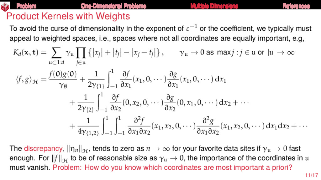
33. Problem One-Dimensional Problems Multiple Dimensions References Product Kernels with Weights To avoid the curse of dimensionality in the exponent of ε−1 or the coefficient, we typically must appeal to weighted spaces, i.e., spaces where not all coordinates are equally important, e.g, Kd(x, t) = u⊂1:d γu j∈u xj + tj − xj − tj , γu → 0 as max j : j ∈ u or |u| → ∞ f, g H = f(0)g(0) γ∅ + 1 2γ{1} 1 −1 ∂f ∂x1 (x1, 0, · · · ) ∂g ∂x1 (x1, 0, · · · ) dx1 + 1 2γ{2} 1 −1 ∂f ∂x2 (0, x2, 0, · · · ) ∂g ∂x2 (0, x1, 0, · · · ) dx2 + · · · + 1 4γ{1,2} 1 −1 1 −1 ∂2f ∂x1∂x2 (x1, x2, 0, · · · ) ∂2g ∂x1∂x2 (x1, x2, 0, · · · ) dx1dx2 + · · · The discrepancy, ηn H , tends to zero as n → ∞ for your favorite data sites if γu → 0 fast enough. For f H to be of reasonable size as γu → 0, the importance of the coordinates in u must vanish. Problem: How do you know which coordinates are most important a priori? 11/17
34. Problem One-Dimensional Problems Multiple Dimensions References These Are a Few of My Favorite Data Sites Good for integration, not sure how good for function approximation Niederreiter, H. Random Number Generation and Quasi-Monte Carlo Methods. (SIAM, Philadelphia, 1992), Sloan, I. H. & Joe, S. Lattice Methods for Multiple Integration. (Oxford University Press, Oxford, 1994), Dick, J. & Pillichshammer, F. Digital Nets and Sequences: Discrepancy Theory and Quasi-Monte Carlo Integration. (Cambridge University Press, Cambridge, 2010). 12/17
35. Problem One-Dimensional Problems Multiple Dimensions References Approximation when Linear Functionals Can Be Evaluated To understand how difficult things can be in higher dimensions, let us make the problem both harder (function approximation) and easier (we can evaluate L(f) for any linear functional L we like). If f(x) = ∞ m=1 fmφm(x) for L2(Ω) orthonormal functions φm, which are simultaneously orthonormal in H with φm H = λ−1 m , and λ1 λ2 · · · , then f H = fm λm ∞ m=1 2 , Kd(x, t) = ∞ m=1 λ2 m φm(x)φm(t), and the optimal algorithm using n linear functionals is f = n m=1 fφm, f − f 2 = fm ∞ m=n+1 2 = fm λm · λm ∞ m=n+1 2 λn+1 f H 13/17
36. Problem One-Dimensional Problems Multiple Dimensions References Approximation when Linear Functionals Can Be Evaluated f(x) = ∞ m=1 fmφm(x), f H = fm λm ∞ m=1 2 , K(x, t) = ∞ m=1 λ2 m φm(x)φm(t), f = n m=1 fφm, f − f 2 = fm ∞ m=n+1 2 = fm λm · λm ∞ m=n+1 2 λn+1 f H If Kd = u⊂1:d γu j∈u ˜ Kj(xj, tj), then the λm and φm are of product form, and bounds on the decay rate of λn+1 in terms of the decay rates of the ˜ λj and the γu are possible. Novak, E. & Woźniakowski, H. Tractability of Multivariate Problems Volume I: Linear Information. EMS Tracts in Mathematics 6 (European Mathematical Society, Zürich, 2008). 14/17
37. Problem One-Dimensional Problems Multiple Dimensions References Approximation when Linear Functionals Can Be Evaluated f(x) = ∞ m=1 fmφm(x), f H = fm λm ∞ m=1 2 , K(x, t) = ∞ m=1 λ2 m φm(x)φm(t), f = n m=1 fφm, f − f 2 = fm ∞ m=n+1 2 = fm λm · λm ∞ m=n+1 2 λn+1 f H If Kd = u⊂1:d γu j∈u ˜ Kj(xj, tj), then the λm and φm are of product form, and bounds on the decay rate of λn+1 in terms of the decay rates of the ˜ λj and the γu are possible. Proposed research direction: Assume f is in the union of unit balls of different weighted Hilbert spaces with most γu vanishing, e.g., γu = 0 for all but O(d) pairs u, so one can hope for n d Use an initial linear functional values to screen for the important coordinate directions. Assume that high order terms do not occur unless lower order terms occur, etc. Use further linear functional values to construct an accurate approximation Novak, E. & Woźniakowski, H. Tractability of Multivariate Problems Volume I: Linear Information. EMS Tracts in Mathematics 6 (European Mathematical Society, Zürich, 2008). 14/17
38. Problem One-Dimensional Problems Multiple Dimensions References How Do We Find a Criteria for Sequential Choice of Data Sites? The existing criteria that for the quality of data sites do not depend on function values. Here is an untried possibility: The error depends on the norm of the function, f H . Although we do not know f H , we can compute the norm of the kriging approximation, f H = yK−1y, which no greater than f H , and perhaps close If you can partition the domain into regions, you can compute f H = yK−1y based on only a subset of the data from a particular region. Place more points where the norm is greater. E.g., region [−1, 0) [0, 1] [−1, 1] f H = yK−1y 4.76 1.87 5.08 15/17
39. Problem One-Dimensional Problems Multiple Dimensions References A Few More Thoughts There is a catalog of Hilbert spaces and their kernels There are connections of low discrepancy designs to traditional designs measures Berlinet, A. & Thomas-Agnan, C. Reproducing Kernel Hilbert Spaces in Probability and Statistics. (Kluwer Academic Publishers, Boston, 2004). H., F. J. & Liu, M. Q. Uniform Designs Limit Aliasing. Biometrika 89, 893–904 (2002). 16/17
40. Thank you
41. Problem One-Dimensional Problems Multiple Dimensions References N. Aronszajn. Theory of Reproducing Kernels. Trans. Amer. Math. Soc. 68, 337–404 (1950). H., F. J. A Generalized Discrepancy and Quadrature Error Bound. Math. Comp. 67, 299–322 (1998). H., F. J. What Affects the Accuracy of Quasi-Monte Carlo Quadrature?. in Monte Carlo and Quasi-Monte Carlo Methods 1998 (eds Niederreiter, H. & Spanier, J.) (Springer-Verlag, Berlin, 2000), 16–55. Novak, E. & Woźniakowski, H. Tractability of Multivariate Problems Volume I: Linear Information. EMS Tracts in Mathematics 6 (European Mathematical Society, Zürich, 2008). Novak, E. & Woźniakowski, H. Tractability of Multivariate Problems Volume II: Standard Information for Functionals. EMS Tracts in Mathematics 12 (European Mathematical Society, Zürich, 2010). 17/17
42. Problem One-Dimensional Problems Multiple Dimensions References Novak, E. & Woźniakowski, H. Tractability of Multivariate Problems: Volume III: Standard Information for Operators. EMS Tracts in Mathematics 18 (European Mathematical Society, Zürich, 2012). Niederreiter, H. Random Number Generation and Quasi-Monte Carlo Methods. (SIAM, Philadelphia, 1992). Sloan, I. H. & Joe, S. Lattice Methods for Multiple Integration. (Oxford University Press, Oxford, 1994). Dick, J. & Pillichshammer, F. Digital Nets and Sequences: Discrepancy Theory and Quasi-Monte Carlo Integration. (Cambridge University Press, Cambridge, 2010). Berlinet, A. & Thomas-Agnan, C. Reproducing Kernel Hilbert Spaces in Probability and Statistics. (Kluwer Academic Publishers, Boston, 2004). H., F. J. & Liu, M. Q. Uniform Designs Limit Aliasing. Biometrika 89, 893–904 (2002). 17/17