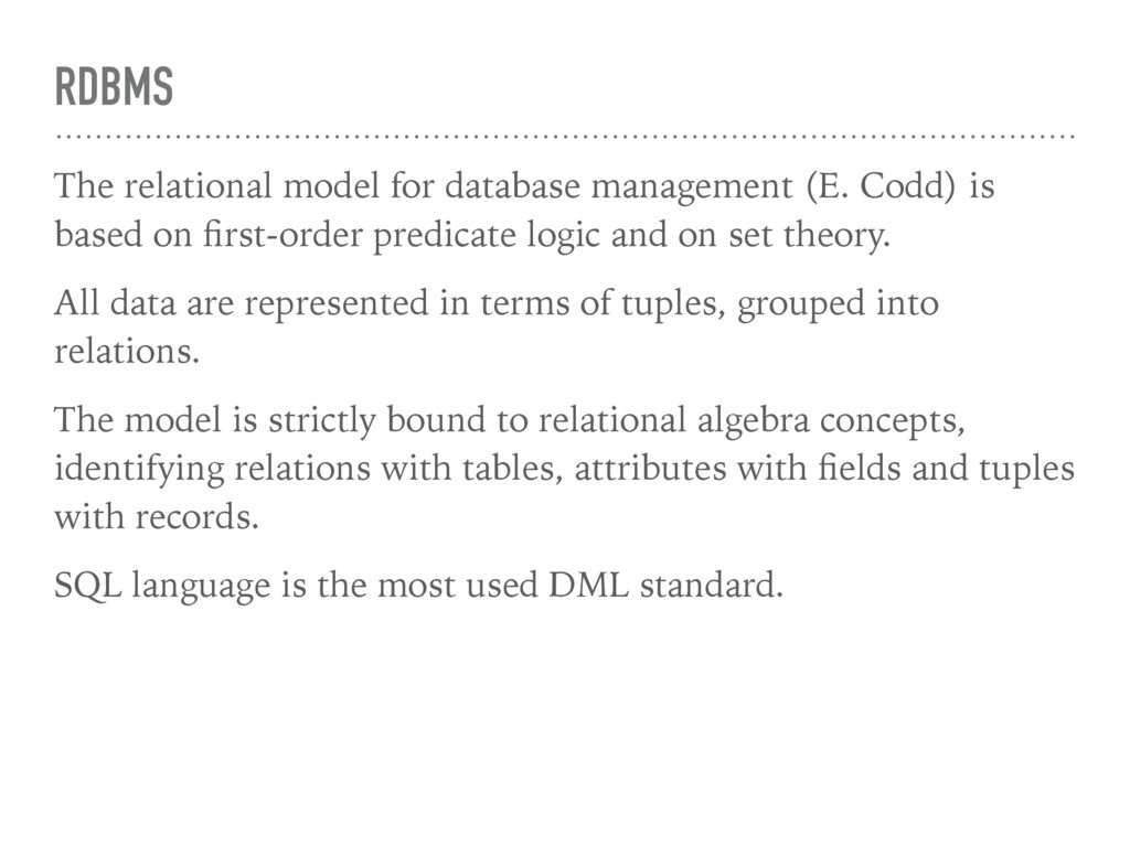
based on first-order predicate logic and on set theory. All data are represented in terms of tuples, grouped into relations. The model is strictly bound to relational algebra concepts, identifying relations with tables, attributes with fields and tuples with records. SQL language is the most used DML standard.
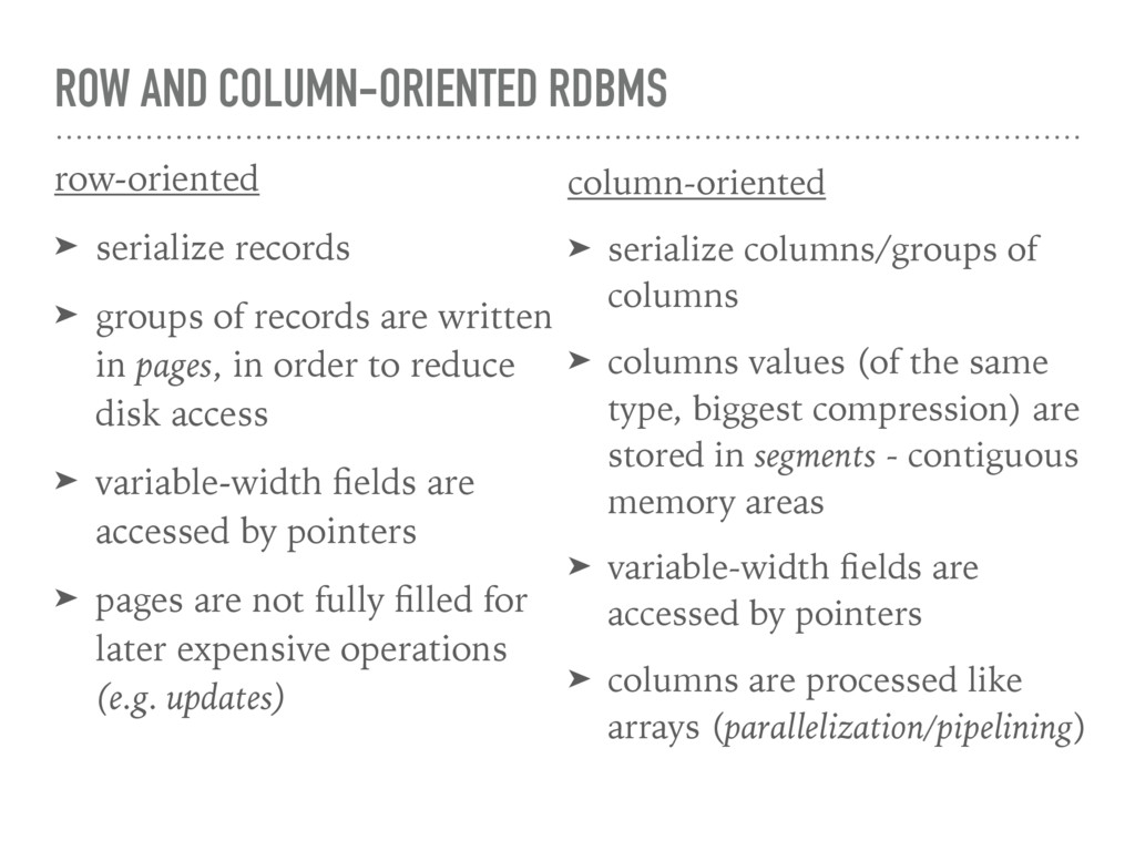
➤ columns values (of the same type, biggest compression) are stored in segments - contiguous memory areas ➤ variable-width fields are accessed by pointers ➤ columns are processed like arrays (parallelization/pipelining) row-oriented ➤ serialize records ➤ groups of records are written in pages, in order to reduce disk access ➤ variable-width fields are accessed by pointers ➤ pages are not fully filled for later expensive operations (e.g. updates)
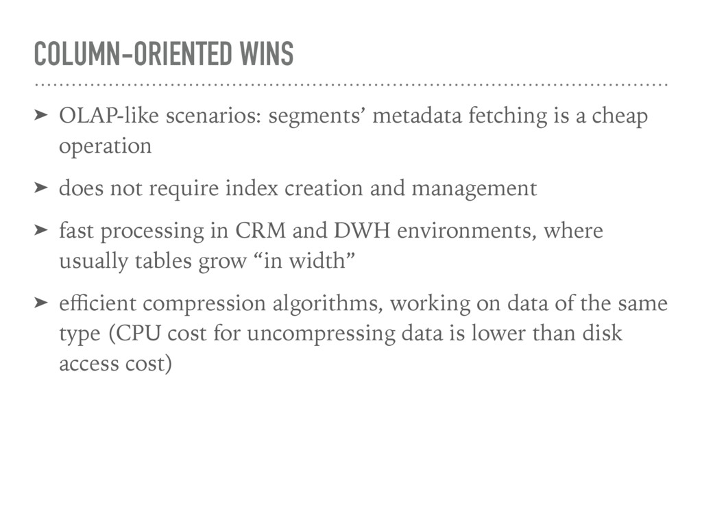
cheap operation ➤ does not require index creation and management ➤ fast processing in CRM and DWH environments, where usually tables grow “in width” ➤ efficient compression algorithms, working on data of the same type (CPU cost for uncompressing data is lower than disk access cost)
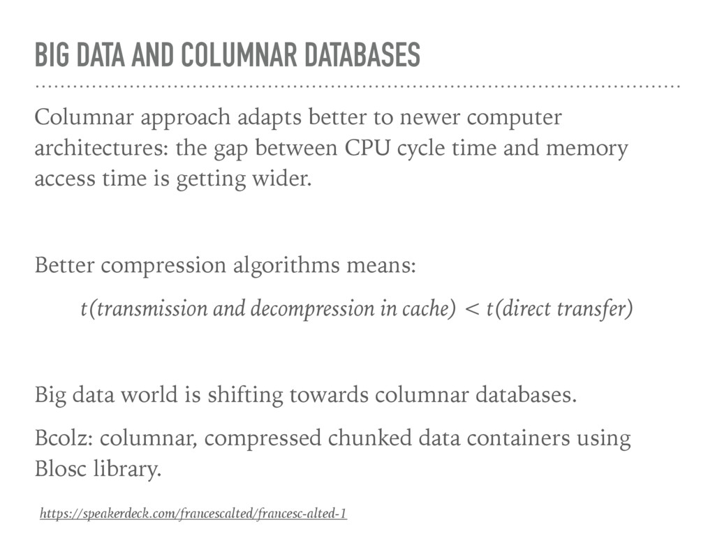
to newer computer architectures: the gap between CPU cycle time and memory access time is getting wider. Better compression algorithms means: t(transmission and decompression in cache) < t(direct transfer) Big data world is shifting towards columnar databases. Bcolz: columnar, compressed chunked data containers using Blosc library.
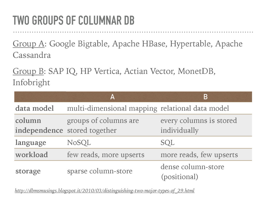
mapping relational data model column independence groups of columns are stored together every columns is stored individually language NoSQL SQL workload few reads, more upserts more reads, few upserts storage sparse column-store dense column-store (positional) http://dbmsmusings.blogspot.it/2010/03/distinguishing-two-major-types-of_29.html Group A: Google Bigtable, Apache HBase, Hypertable, Apache Cassandra Group B: SAP IQ, HP Vertica, Actian Vector, MonetDB, Infobright
Wiskunde & Informatica (CWI) of Amsterdam. The MonetDB team is pioneering column-store technologies since 1993, the first official open-source release of MonetDB was in the year 2004. MonetDB purpose is to deliver high performance throughput in different applications: data mining, BI, OLAP , scientific databases, text/BLOB retrieval, GIS, etc.
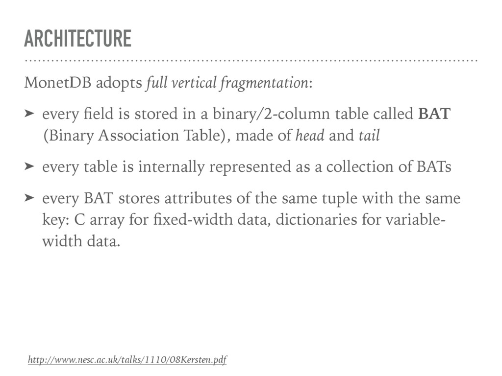
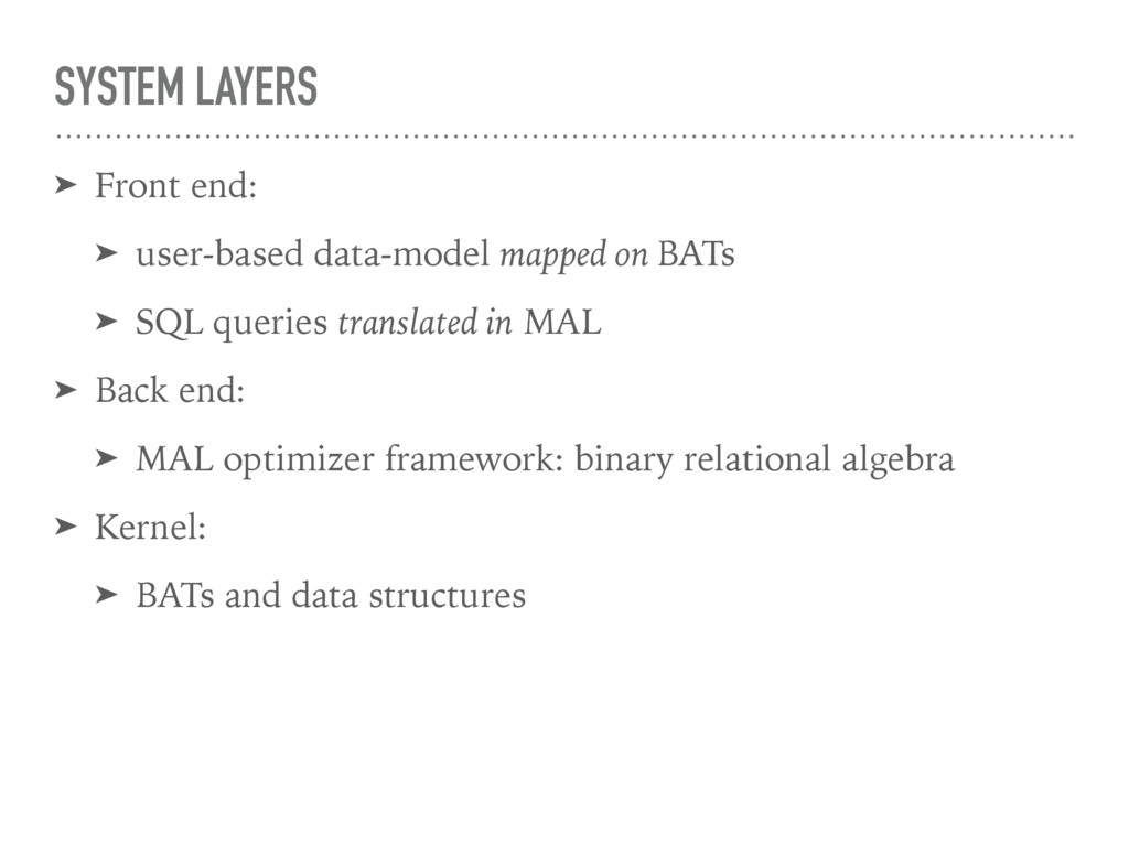
is stored in a binary/2-column table called BAT (Binary Association Table), made of head and tail ➤ every table is internally represented as a collection of BATs ➤ every BAT stores attributes of the same tuple with the same key: C array for fixed-width data, dictionaries for variable- width data.
(MonetDB Assembly Language) ➤ complex operations are decomposed in simpler sequences of MAL relational algebra operators, that can be executed on the whole column.
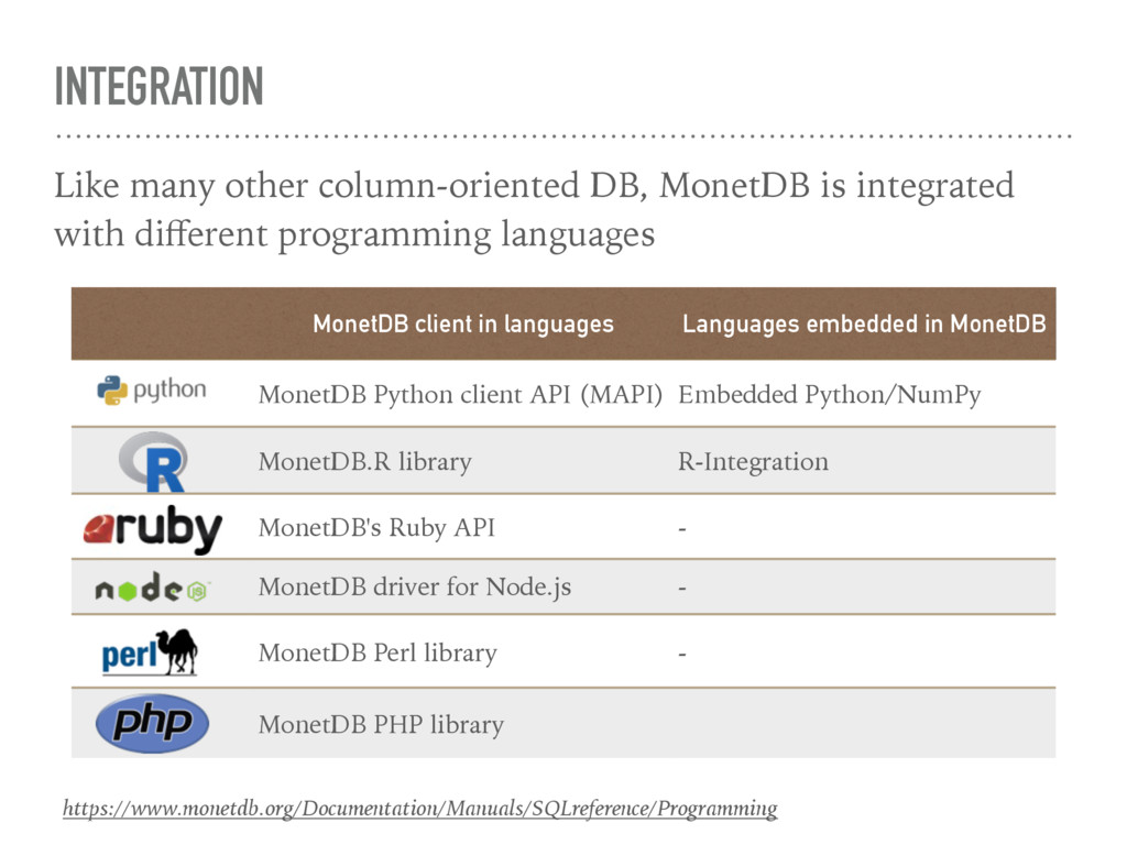
Python client API (MAPI) Embedded Python/NumPy MonetDB.R library R-Integration MonetDB's Ruby API - MonetDB driver for Node.js - MonetDB Perl library - MonetDB PHP library https://www.monetdb.org/Documentation/Manuals/SQLreference/Programming Like many other column-oriented DB, MonetDB is integrated with different programming languages
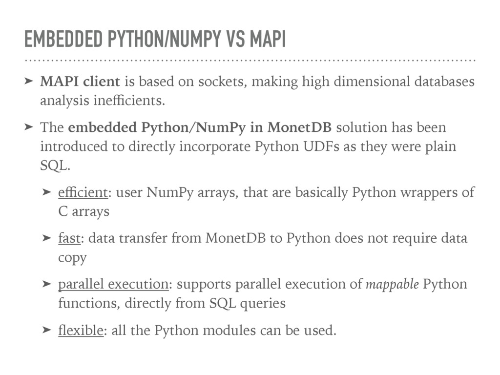
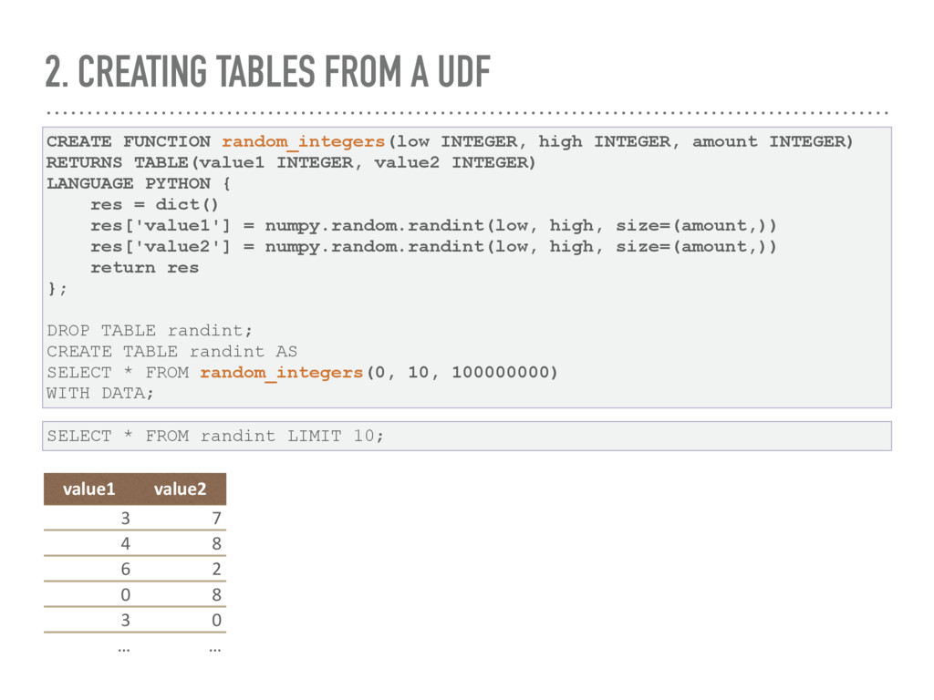
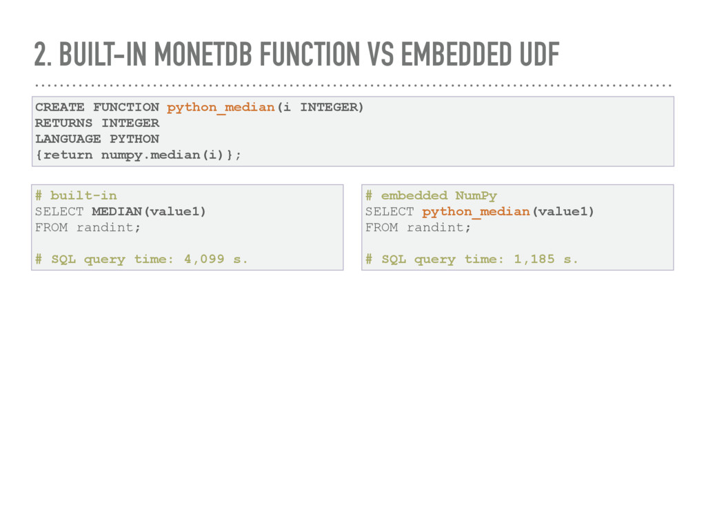
sockets, making high dimensional databases analysis inefficients. ➤ The embedded Python/NumPy in MonetDB solution has been introduced to directly incorporate Python UDFs as they were plain SQL. ➤ efficient: user NumPy arrays, that are basically Python wrappers of C arrays ➤ fast: data transfer from MonetDB to Python does not require data copy ➤ parallel execution: supports parallel execution of mappable Python functions, directly from SQL queries ➤ flexible: all the Python modules can be used.
by splitting columns and executing queries in parallel, on different threads. ➤ Not all queries can be executed in parallel, some of them require full column access. These are called blocking operations, the default for embedded Python/NumPy UDFs.
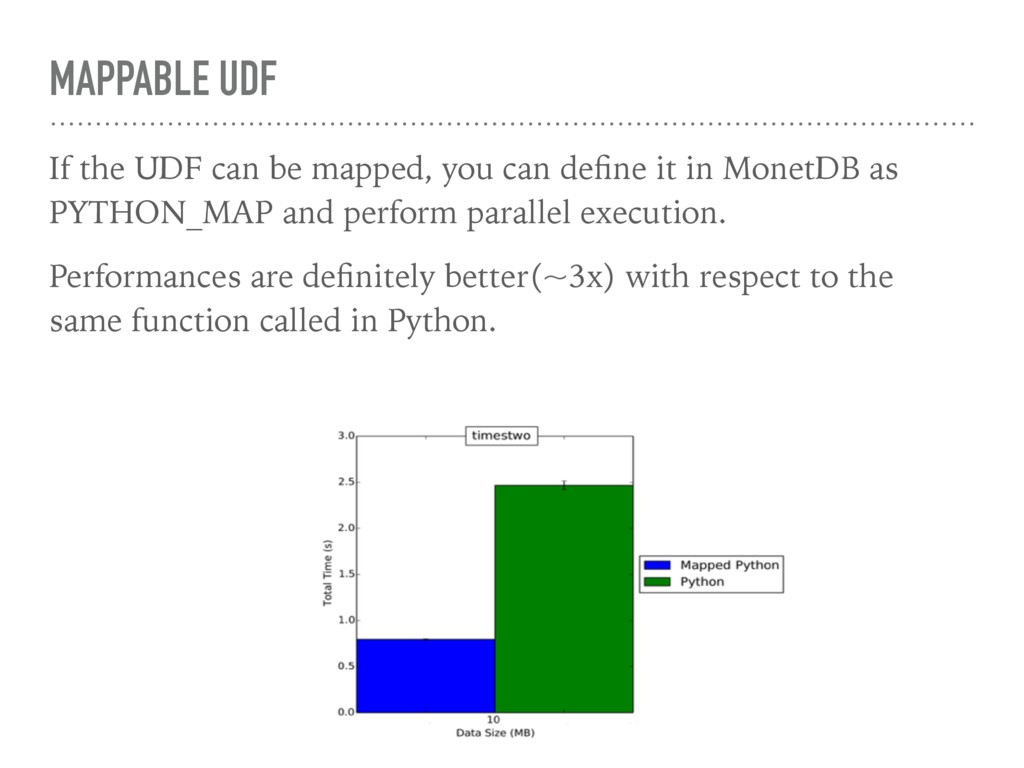
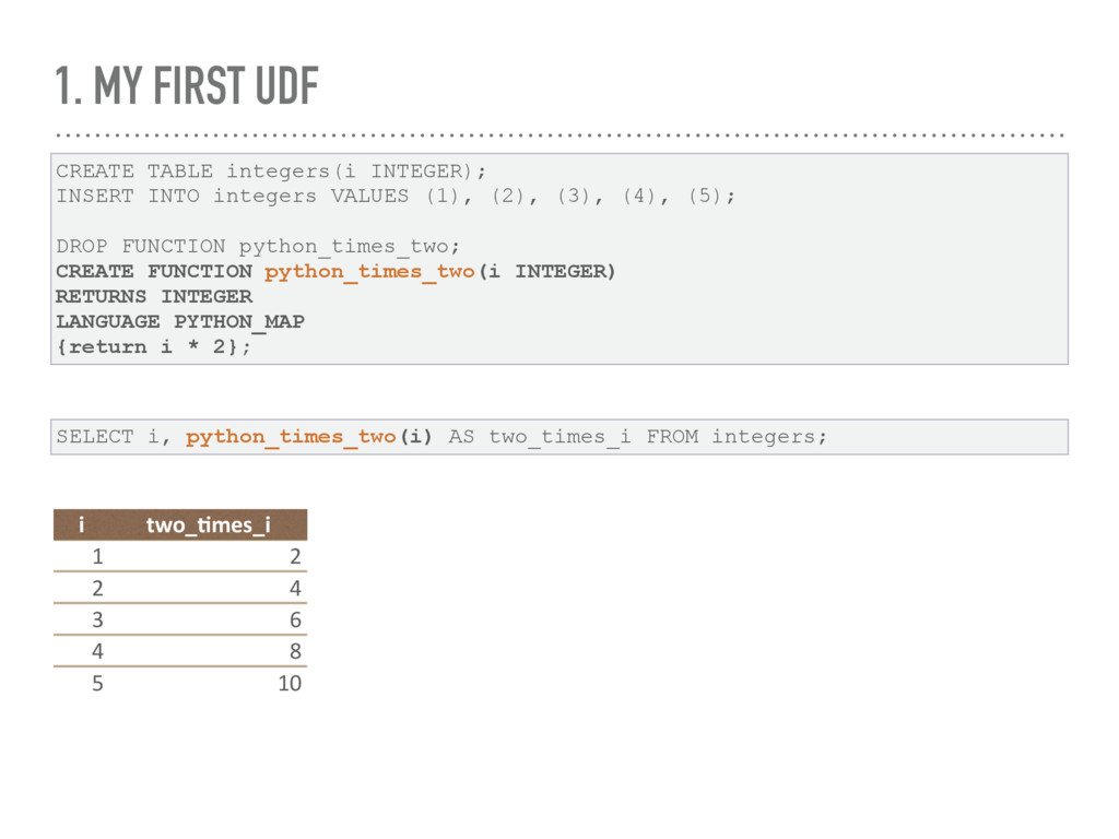
define it in MonetDB as PYTHON_MAP and perform parallel execution. Performances are definitely better(~3x) with respect to the same function called in Python.
integers VALUES (1), (2), (3), (4), (5); DROP FUNCTION python_times_two; CREATE FUNCTION python_times_two(i INTEGER) RETURNS INTEGER LANGUAGE PYTHON_MAP {return i * 2}; SELECT i, python_times_two(i) AS two_times_i FROM integers; i two_&mes_i 1 2 2 4 3 6 4 8 5 10
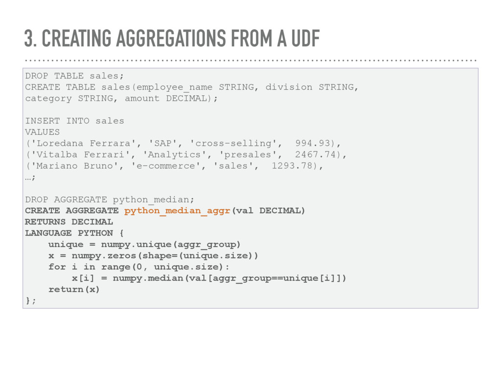
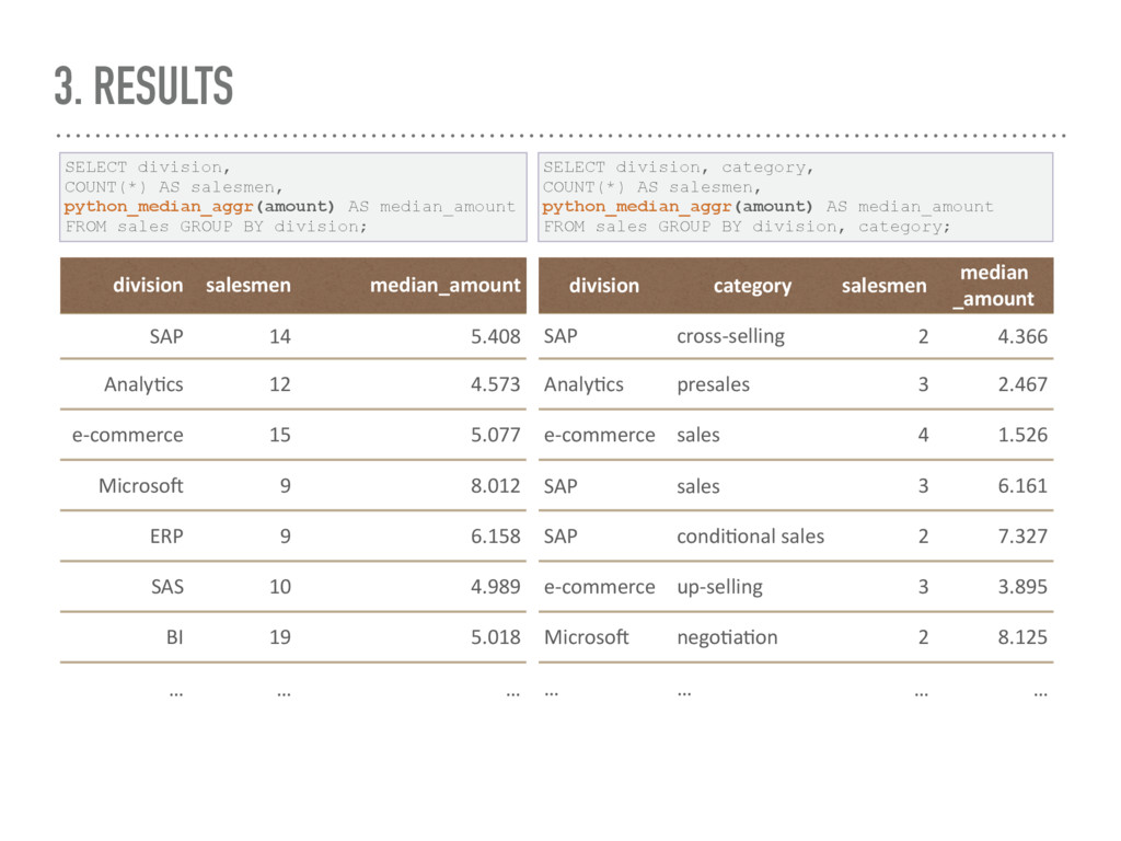
to perform complex operations on datasets/tables. NumPy and Scikit-learn allow the application of machine learning techniques on data. The best performances are obtained using embedded Python/ NumPy UDFs in MonetDB.
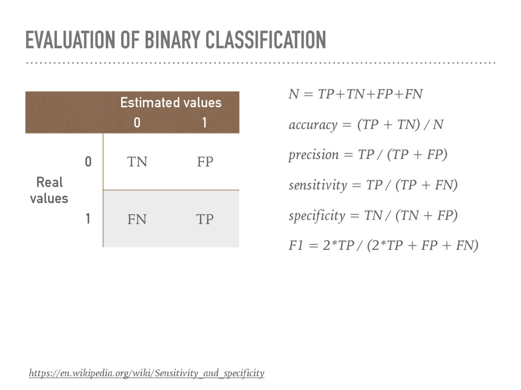
sector operating exclusively in B2B, normal-trade channel. It plans promotions in favor of final customers, involving retailers. There are two main goals related to the promotions: ➤ the company is interested in estimating the quantity of gadgets to buy in order to satisfy the request ➤ the agents want to know if a retailer is interested in being involved in the promotion. We are facing a binary classification problem: the retailer partecipates/doesn’t partecipate in a promotion.
that counts about 120M rows in a 2 year period. ➤ We created and enriched a CRM table with 43.000 records/ retailers and about 150 features, where we observe the target variable: taking part in the promotion. ➤ The features are heterogeneous and related to: retailer category, economic behaviour (wrt to brand and product line), historical sales volumes, credit exposures, localization, attendance at previous promotions, RFM, etc.
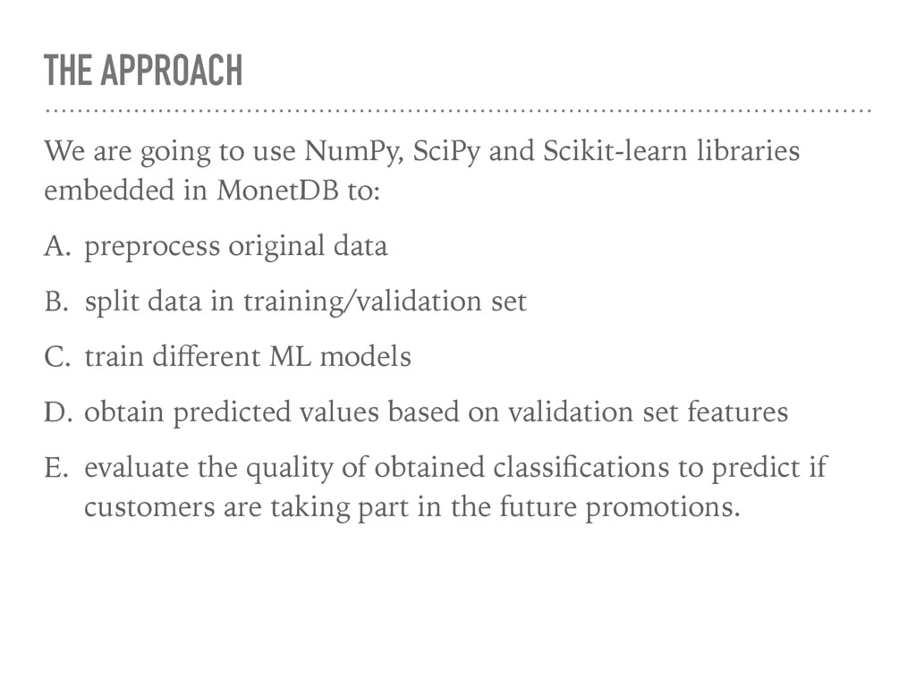
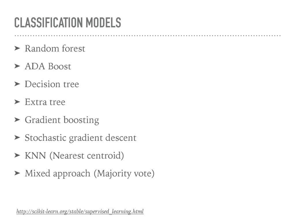
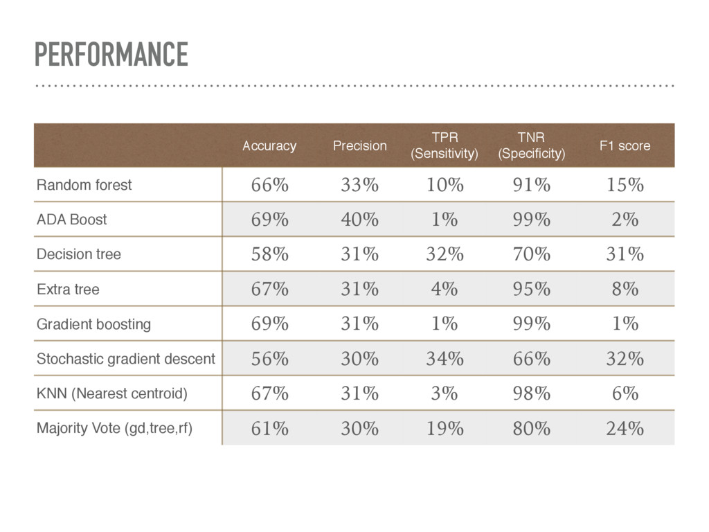
Scikit-learn libraries embedded in MonetDB to: A. preprocess original data B. split data in training/validation set C. train different ML models D. obtain predicted values based on validation set features E. evaluate the quality of obtained classifications to predict if customers are taking part in the future promotions.
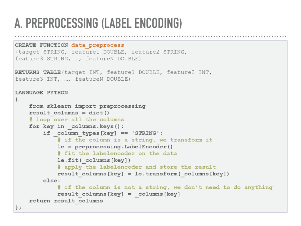
DOUBLE, feature2 STRING, feature3 STRING, …, featureN DOUBLE) RETURNS TABLE(target INT, feature1 DOUBLE, feature2 INT, feature3 INT, …, featureN DOUBLE) LANGUAGE PYTHON { from sklearn import preprocessing result_columns = dict() # loop over all the columns for key in _columns.keys(): if _column_types[key] == 'STRING': # if the column is a string, we transform it le = preprocessing.LabelEncoder() # fit the labelencoder on the data le.fit(_columns[key]) # apply the labelencoder and store the result result_columns[key] = le.transform(_columns[key]) else: # if the column is not a string, we don't need to do anything result_columns[key] = _columns[key] return result_columns };
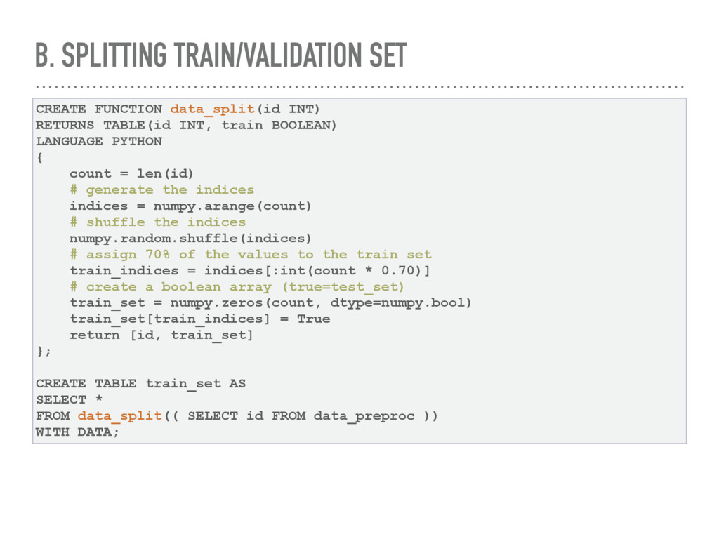
INT, train BOOLEAN) LANGUAGE PYTHON { count = len(id) # generate the indices indices = numpy.arange(count) # shuffle the indices numpy.random.shuffle(indices) # assign 70% of the values to the train set train_indices = indices[:int(count * 0.70)] # create a boolean array (true=test_set) train_set = numpy.zeros(count, dtype=numpy.bool) train_set[train_indices] = True return [id, train_set] }; CREATE TABLE train_set AS SELECT * FROM data_split(( SELECT id FROM data_preproc )) WITH DATA;
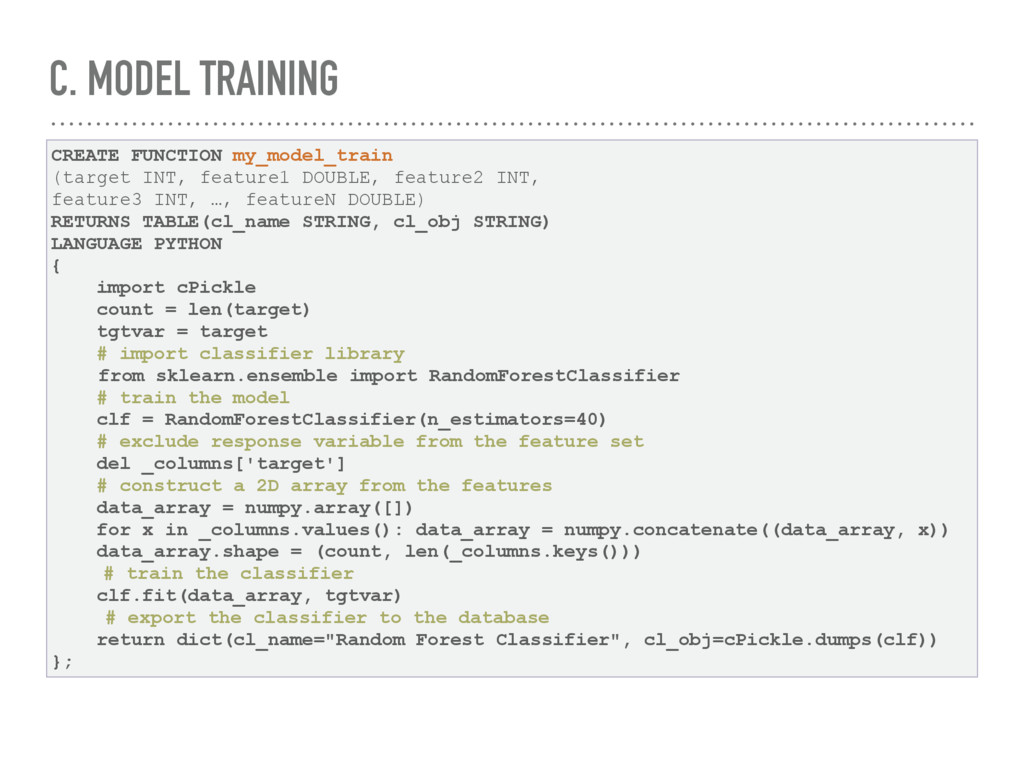
feature2 INT, feature3 INT, …, featureN DOUBLE) RETURNS TABLE(cl_name STRING, cl_obj STRING) LANGUAGE PYTHON { import cPickle count = len(target) tgtvar = target # import classifier library from sklearn.ensemble import RandomForestClassifier # train the model clf = RandomForestClassifier(n_estimators=40) # exclude response variable from the feature set del _columns['target'] # construct a 2D array from the features data_array = numpy.array([]) for x in _columns.values(): data_array = numpy.concatenate((data_array, x)) data_array.shape = (count, len(_columns.keys())) # train the classifier clf.fit(data_array, tgtvar) # export the classifier to the database return dict(cl_name="Random Forest Classifier", cl_obj=cPickle.dumps(clf)) };
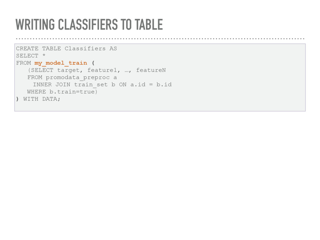
FROM my_model_train ( (SELECT target, feature1, …, featureN FROM promodata_preproc a INNER JOIN train_set b ON a.id = b.id WHERE b.train=true) ) WITH DATA;
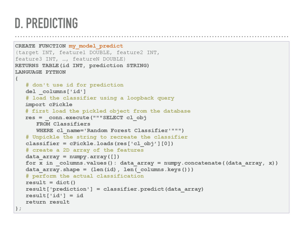
INT, feature3 INT, …, featureN DOUBLE) RETURNS TABLE(id INT, prediction STRING) LANGUAGE PYTHON { # don't use id for prediction del _columns['id'] # load the classifier using a loopback query import cPickle # first load the pickled object from the database res = _conn.execute("""SELECT cl_obj FROM Classifiers WHERE cl_name='Random Forest Classifier'""") # Unpickle the string to recreate the classifier classifier = cPickle.loads(res['cl_obj’][0]) # create a 2D array of the features data_array = numpy.array([]) for x in _columns.values(): data_array = numpy.concatenate((data_array, x)) data_array.shape = (len(id), len(_columns.keys())) # perform the actual classification result = dict() result['prediction'] = classifier.predict(data_array) result['id'] = id return result };
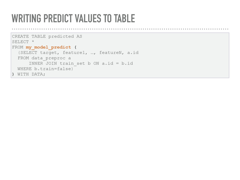
* FROM my_model_predict ( (SELECT target, feature1, …, featureN, a.id FROM data_preproc a INNER JOIN train_set b ON a.id = b.id WHERE b.train=false) ) WITH DATA;
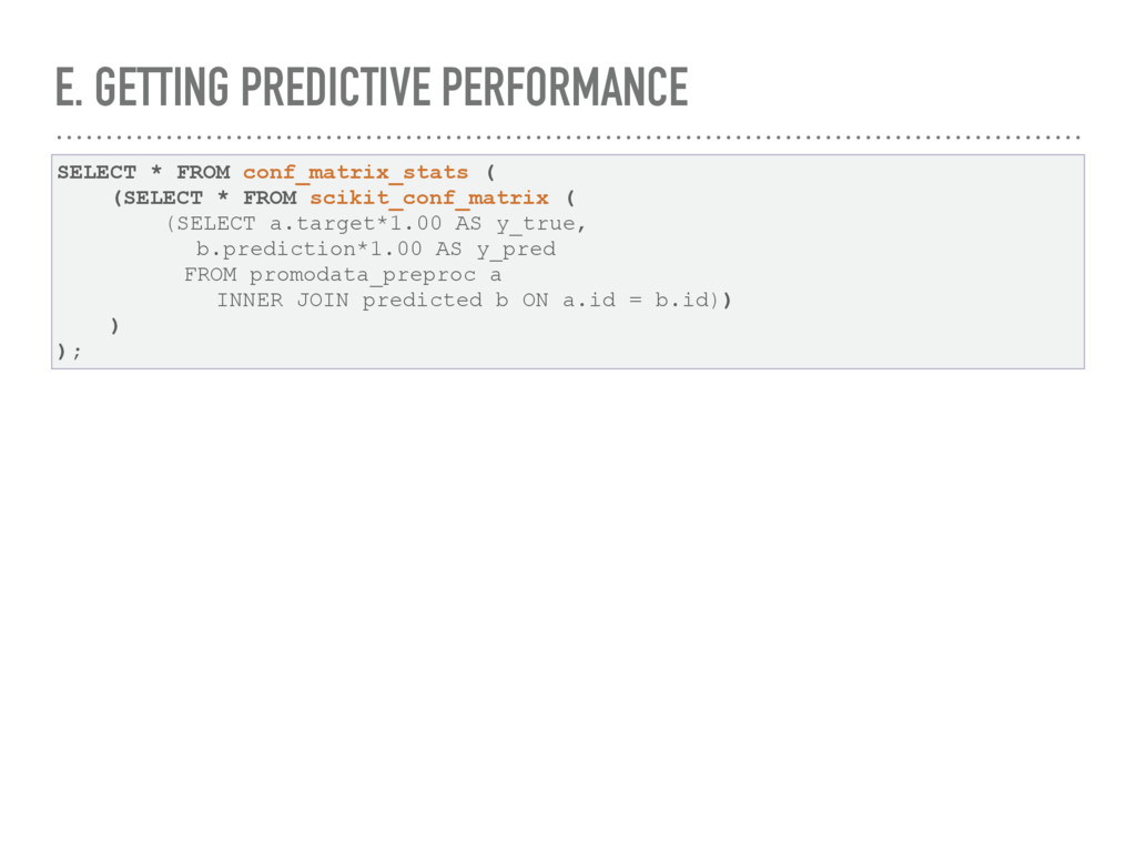
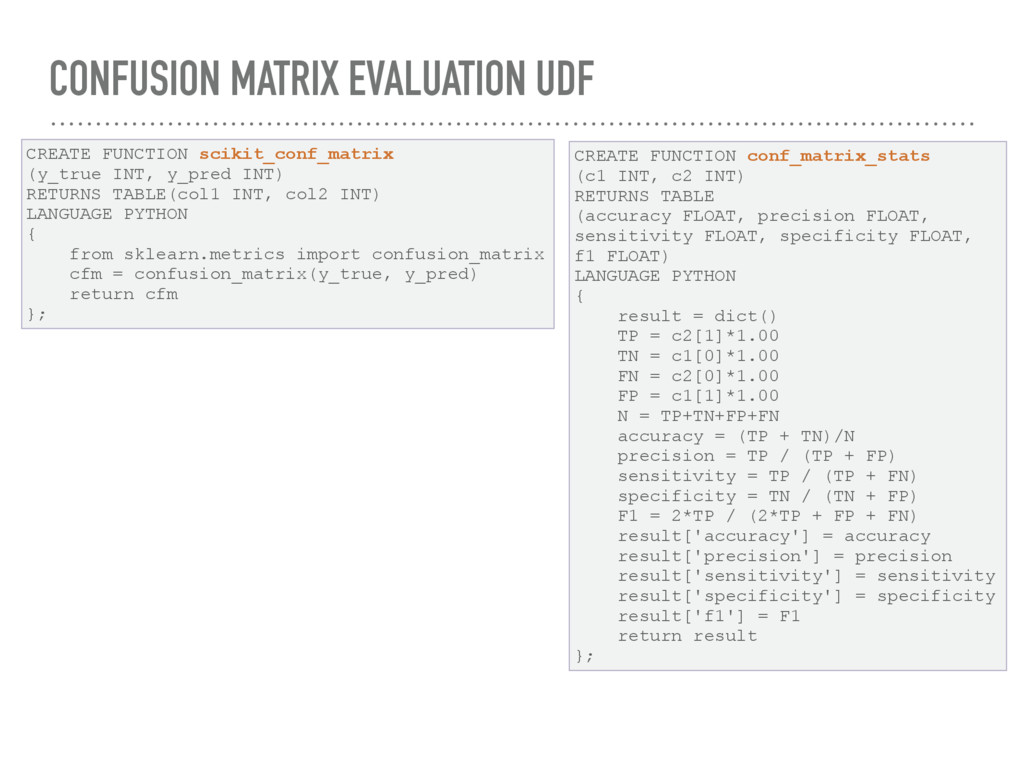
* FROM scikit_conf_matrix ( (SELECT a.target*1.00 AS y_true, b.prediction*1.00 AS y_pred FROM promodata_preproc a INNER JOIN predicted b ON a.id = b.id)) ) );