Using potential vorticity and its attendant theorems to study the subtropical thermocline water mass

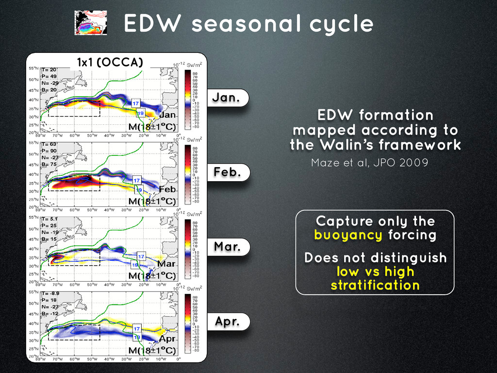
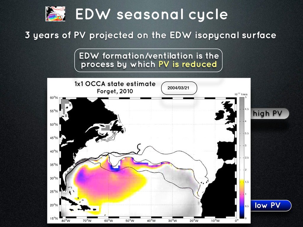
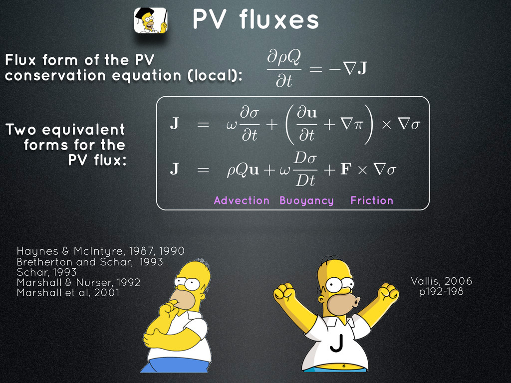
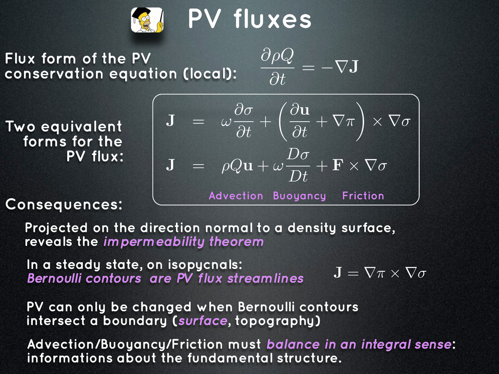
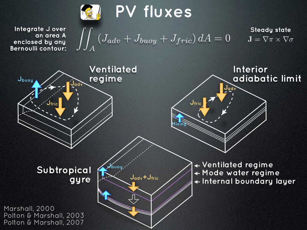
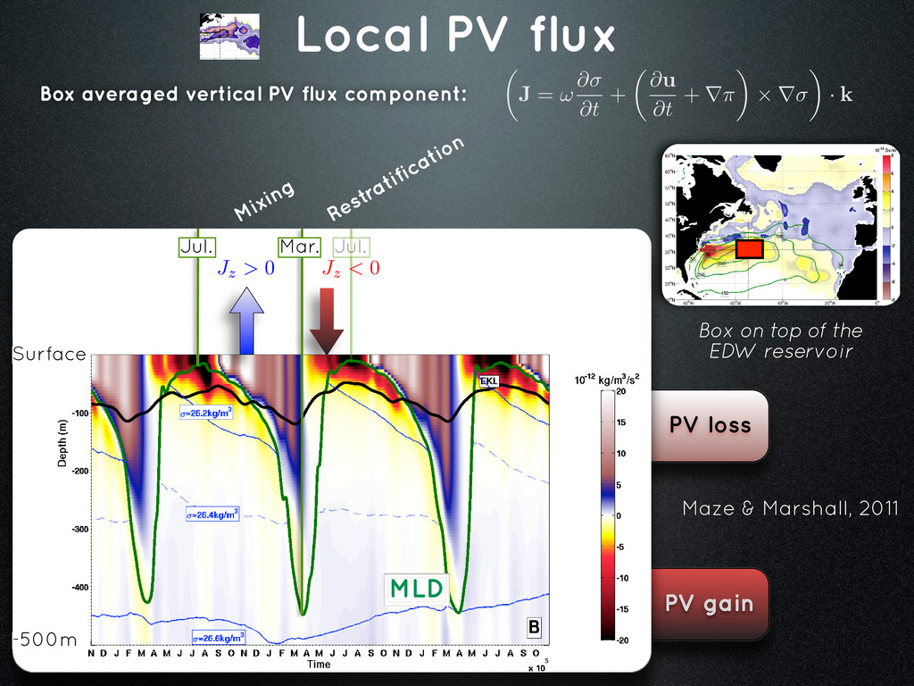
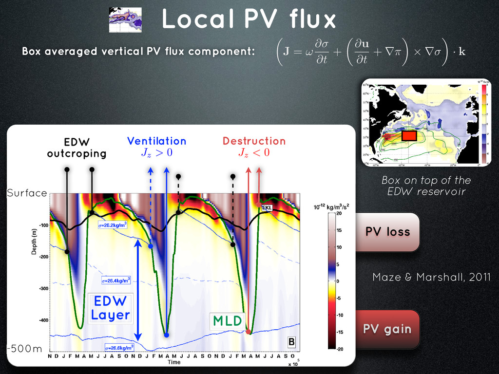
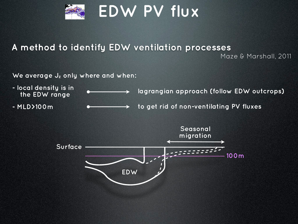
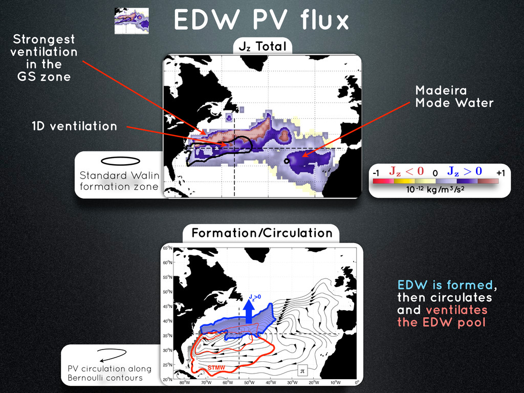
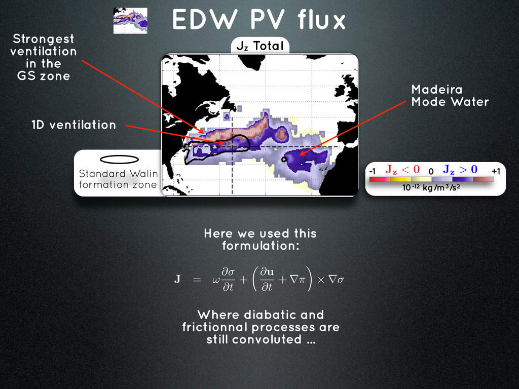
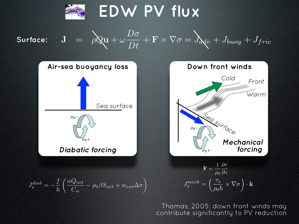
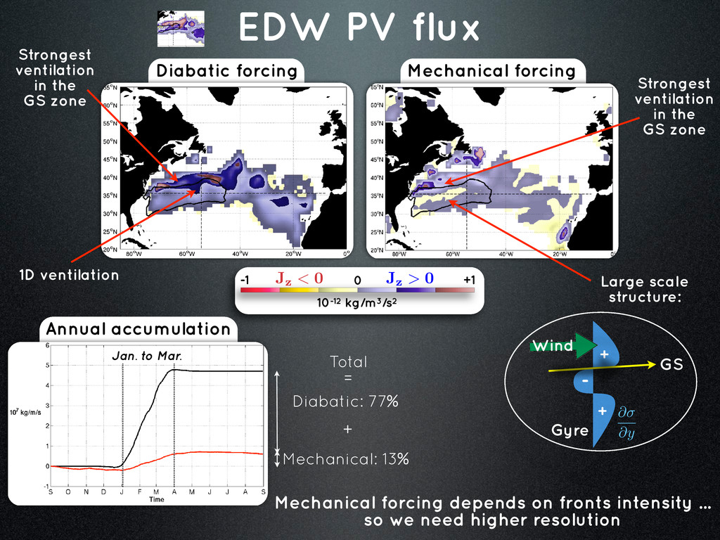
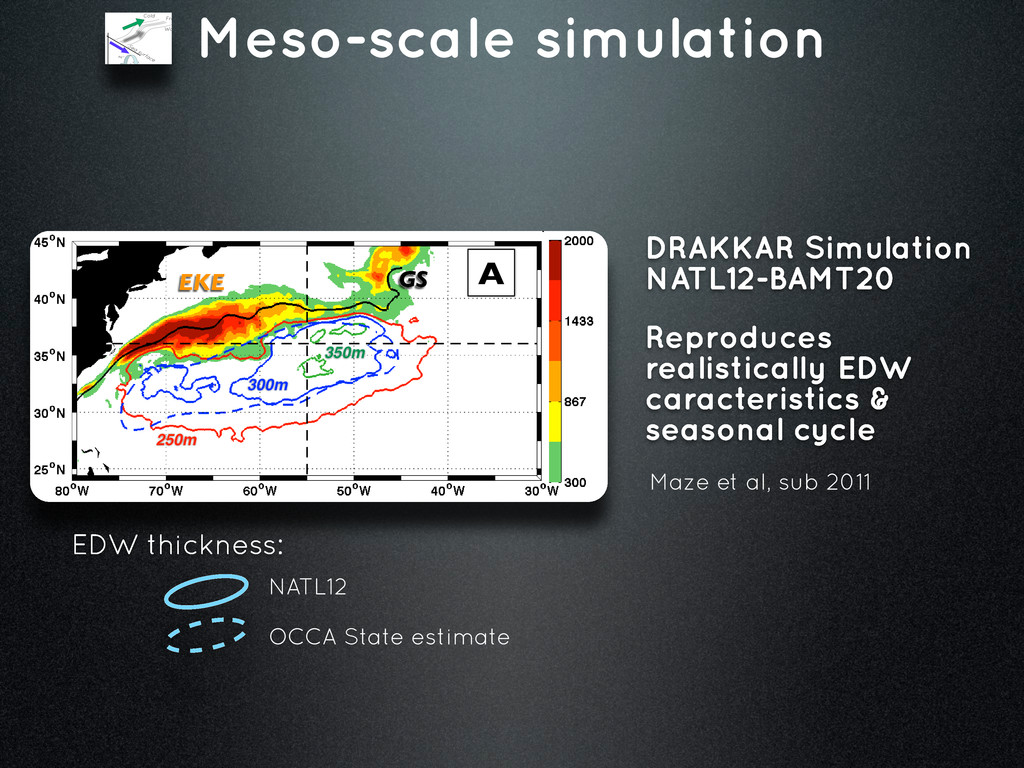
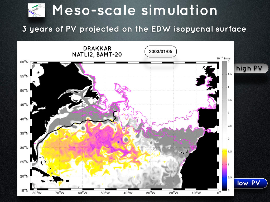
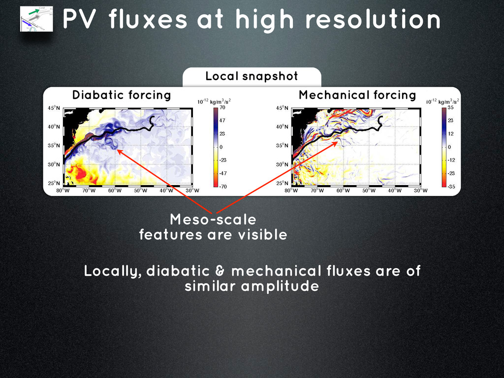
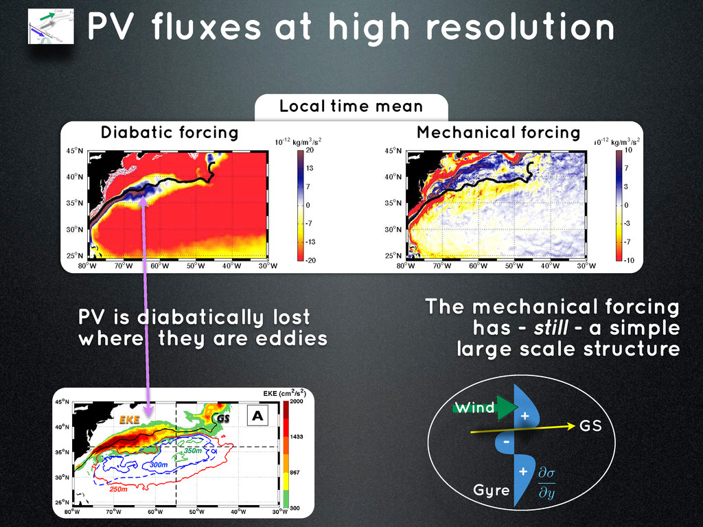
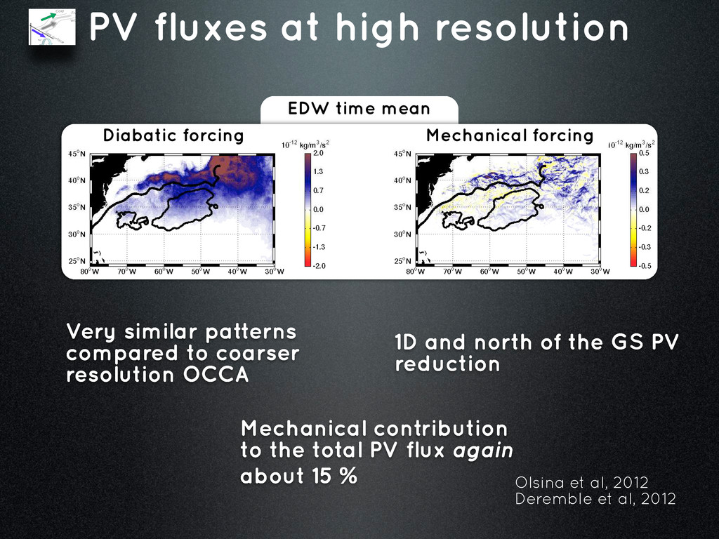
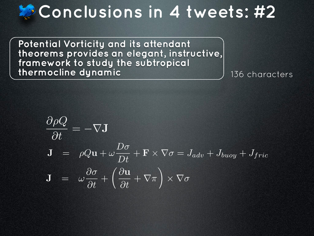
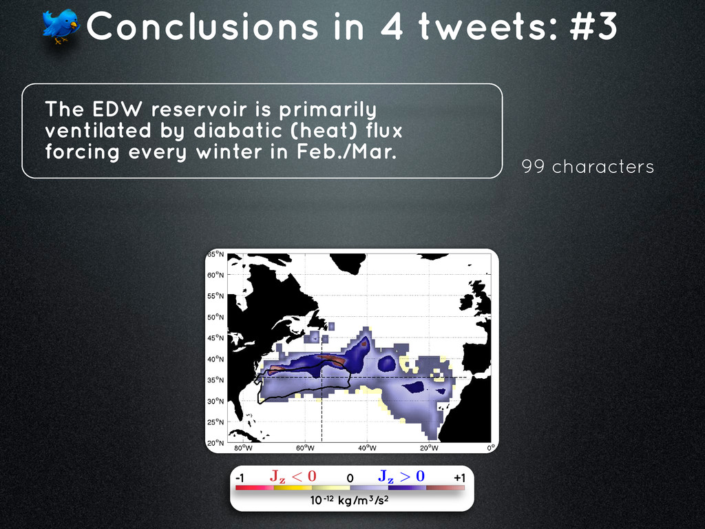
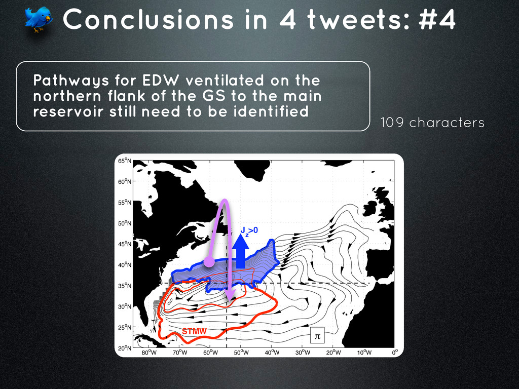
Potential vorticity (PV) fluxes are a great tool to investigate surface water mass dynamic in subtropical gyres. Analyzed fields of ocean circulation and the flux form of the potential vorticity equation will be used to map the creation and subsequent circulation of low potential vorticity waters known as Subtropical Mode Water (STMW) in the North Atlantic. Results from a coarse resolution ocean state estimate (1x1) constrained by data assimilation and from a forward meso-scale eddy resolving numerical simulation (1/12) will be shown and compared. A novel mapping technique to (i) render the seasonal cycle and annual-mean mixed layer vertical flux of potential vorticity through outcrops and (ii) visualize the extraction of PV from the mode water layer in winter, over and to the south of the Gulf Stream will be presented. We will show that both buoyancy loss and wind forcing contribute to the extraction of PV (and thus formation of mode water) but that the former greatly exceeds the latter. The subsequent path of STMW will also be mapped using Bernoulli contours on isopycnal surfaces.

Transcript

1. Using potential vorticity and its attendant theorems to study the subtropical thermocline water mass Guillaume Maze & John Marshall Julie Deshayes (Ifremer, LPO) (MIT) (CNRS, LPO)
2. 60˚W 0˚ 60˚E 120˚E 80˚S 60˚ 40˚ 20˚ 0˚ 20˚ 40˚ 60˚ 80˚N 26.9–27.75 26.5–26.8 26.2–26.7 26.2–26.3 26.5 25.5 26.85 26.0 27.1 26.9–27.75 26.5–26.8 26.2–26.7 26.2–26.3 26.5 25.5 26.85 26.0 27.1 (a) Outline Introduction J PV fluxes EDW seas. cyc. Meso-scale ? Jz and EDW cycle Conclusions
3. The subtropical thermocline is the natural barrier between water masses ventilated efficiently but with different time scales Subtropical thermocline Plate 5.4.3 (a) Mode water distributions in the world’s oceans, after Talley (1999a). Red coloured areas show the subtropical mode waters (STMWs) associated with the subtropical western boundary currents in each ocean (the first type). Purple coloured areas show the eastern type of subtropical mode waters (the second type), including Madeira Mode Water, North Pacific Eastern STMW and South Pacific Eastern STMW. Brown coloured areas show the third type of subtropical and subpolar mode waters, including North Atlantic Subpolar Mode Water, Subantarctic Mode Water and North Pacific Central Mode Water. Approximate potential densities (!0 ) are indicated. Black arrows denote the subtropical gyre circulation. See the text for explanation for each type of mode water. (b) Low-salinity intermediate water distributions in the world’s oceans, after Talley (1999a). Shown are the North Pacific Intermediate Water (light green), Antarctic Intermediate Water (green), overlap of NPIW and AAIW (medium green), and Labrador Sea Water (blue).The location of formation for each intermediate water is shown with an X. Regions of strong mixing near the ventilation sources that strongly affect the characteristics of the new intermediate waters are shown with cross-hatching. 60˚W 0˚ 60˚E 120˚E 180˚ 120˚W 80˚S 60˚ 40˚ 20˚ 0˚ 20˚ 40˚ 60˚ 80˚N 26.9–27.75 26.5–26.8 26.2–26.7 26.2–26.3 26.5 25.2 25.5 25.5 26.2 26.85 26.0 27.1 26.0 24–25.4 26.9–27.75 26.5–26.8 26.2–26.7 26.2–26.3 26.5 25.2 25.5 25.5 26.2 26.85 26.0 27.1 26.0 24–25.4 60˚W 0˚ 60˚E 120˚E 180˚ 120˚W 80˚S 60˚ 40˚ 20˚ 0˚ 20˚ 40˚ 60˚ 80˚N + + + (a) (b) Pole Equator Gulf Stream Ventilation Subduction Circulation Schematic view for the North Atlantic
4. 60˚W 0˚ 60˚E 120˚E 180˚ 120˚W 80˚S 60˚ 40˚ 20˚ 0˚ 20˚ 40˚ 60˚ 80˚N 26.9–27.75 26.5–26.8 26.2–26.7 26.2–26.3 26.5 25.2 25.5 25.5 26.2 26.85 26.0 27.1 26.0 24–25.4 26.9–27.75 26.5–26.8 26.2–26.7 26.2–26.3 26.5 25.2 25.5 25.5 26.2 26.85 26.0 27.1 26.0 24–25.4 (a) Thermocline water mass Hanawa & Talley (2001) Thick layer ie. mode waters, on equator flank of western boundary currents Challenger, 1873 Near-Surface layer: above the main thermocline Plate 5.4.3 (a) Mode water distributions in the world’s oceans, after Talley (1999a). Red coloured areas show the subtropical mode waters (STMWs) associated with the subtropical western boundary currents in each ocean (the first type). Purple coloured areas show the eastern type of subtropical mode waters (the second type), including Madeira Mode Water, North Pacific Eastern STMW and South Pacific Eastern STMW. Brown coloured areas show the third type of subtropical and subpolar mode waters, including North Atlantic Subpolar Mode Water, Subantarctic Mode Water and North Pacific Central Mode Water. Approximate potential densities (!0 ) are indicated. Black arrows denote the subtropical gyre circulation. See the text for explanation for each type of mode water. (b) Low-salinity intermediate water distributions in the world’s oceans, after Talley (1999a). Shown are the North Pacific Intermediate Water (light green), Antarctic Intermediate Water (green), overlap of NPIW and AAIW (medium green), and Labrador Sea Water (blue).The location of formation for each intermediate water is shown with an X. Regions of strong mixing near the ventilation sources that strongly affect the characteristics of the new intermediate waters are shown with cross-hatching. 60˚W 0˚ 60˚E 120˚E 180˚ 120˚W 80˚S 60˚ 40˚ 20˚ 0˚ 20˚ 40˚ 60˚ 80˚N 26.9–27.75 26.5–26.8 26.2–26.7 26.2–26.3 26.5 25.2 25.5 25.5 26.2 26.85 26.0 27.1 26.0 24–25.4 26.9–27.75 26.5–26.8 26.2–26.7 26.2–26.3 26.5 25.2 25.5 25.5 26.2 26.85 26.0 27.1 26.0 24–25.4 60˚W 0˚ 60˚E 120˚E 180˚ 120˚W 80˚S 60˚ 40˚ 20˚ 0˚ 20˚ 40˚ 60˚ 80˚N + + + (a) (b) Ventilation time scale: 3-10 years
5. Why do we care ? Plate 5.4.3 (a) Mode water distributions in the world’s oceans, after Talley (1999a). Red coloured areas show the subtropical mode waters (STMWs) associated with the subtropical western boundary currents in each ocean (the first type). Purple coloured areas show the eastern type of subtropical mode waters (the second type), including Madeira Mode Water, North Pacific Eastern STMW and South Pacific Eastern STMW. Brown coloured areas show the third type of subtropical and subpolar mode waters, including North Atlantic Subpolar Mode Water, Subantarctic Mode Water and North Pacific Central Mode Water. Approximate potential densities (!0 ) are indicated. Black arrows denote the subtropical gyre circulation. See the text for explanation for each type of mode water. (b) Low-salinity intermediate water distributions in the world’s oceans, after Talley (1999a). Shown are the North Pacific Intermediate Water (light green), Antarctic Intermediate Water (green), overlap of NPIW and AAIW (medium green), and Labrador Sea Water (blue).The location of formation for each intermediate water is shown with an X. Regions of strong mixing near the ventilation sources that strongly affect the characteristics of the new intermediate waters are shown with cross-hatching. 60˚W 0˚ 60˚E 120˚E 180˚ 120˚W 80˚S 60˚ 40˚ 20˚ 0˚ 20˚ 40˚ 60˚ 80˚N 26.9–27.75 26.5–26.8 26.2–26.7 26.2–26.3 26.5 25.2 25.5 25.5 26.2 26.85 26.0 27.1 26.0 24–25.4 26.9–27.75 26.5–26.8 26.2–26.7 26.2–26.3 26.5 25.2 25.5 25.5 26.2 26.85 26.0 27.1 26.0 24–25.4 60˚W 0˚ 60˚E 120˚E 180˚ 120˚W 80˚S 60˚ 40˚ 20˚ 0˚ 20˚ 40˚ 60˚ 80˚N + + + (a) (b) Observed heat content tendancy in the Atlantic Period: 1955-2003, in 108 J/yr Levitus & Boyer, 2005 -80 -60 -40 -20 0 20 40 60 80 Latitude -80 -60 -40 -20 0 20 40 60 80 Latitude 1450 1250 1050 850 650 450 250 50 Depth (meters) 1450 1250 1050 850 650 450 250 50 Depth (meters) T➚ T➘ +5 +4 +1 -80 -60 -40 -20 0 20 40 60 80 Latitude -80 -60 -40 -20 0 20 40 60 80 Latitude 1450 1250 1050 850 650 450 250 50 Depth (meters) 1450 1250 1050 850 650 450 250 50 Depth (meters) T➚ T➘ +5 +4 +1 The climatic signal is constrained: - by the thermocline - to the mode water layer North South Eq. North South Eq. Thermocline in WOA
6. Kelly et al, JC 2010 Dong & Kelly, JPO 2004 Increased GS heat transport Larger heat content Small EDW Deeper thermocline ? Decreased GS heat transport Smaller heat content Larger EDW Shallower thermocline ? Why do we care ? Intense air-sea exchange where ocean gives up heat to the atmosphere Subtropical gyre Eq. Pole Heat T ransport WBC Ocean-Atmosphere transfert zone Total Atmosphere Ocean Plate 5.4.3 (a) Mode water distributions in the world’s oceans, after Talley (1999a). Red coloured areas show the subtropical mode waters (STMWs) associated with the subtropical western boundary currents in each ocean (the first type). Purple coloured areas show the eastern type of subtropical mode waters (the second type), including Madeira Mode Water, North Pacific Eastern STMW and South Pacific Eastern STMW. Brown coloured areas show the third type of subtropical and subpolar mode waters, including North Atlantic Subpolar Mode Water, Subantarctic Mode Water and North Pacific Central Mode Water. Approximate potential densities (!0 ) are indicated. Black arrows denote the subtropical gyre circulation. See the text for explanation for each type of mode water. (b) Low-salinity intermediate water distributions in the world’s oceans, after Talley (1999a). Shown are the North Pacific Intermediate Water (light green), Antarctic Intermediate Water (green), overlap of NPIW and AAIW (medium green), and Labrador Sea Water (blue).The location of formation for each intermediate water is shown with an X. Regions of strong mixing near the ventilation sources that strongly affect the characteristics of the new intermediate waters are shown with cross-hatching. 60˚W 0˚ 60˚E 120˚E 180˚ 120˚W 80˚S 60˚ 40˚ 20˚ 0˚ 20˚ 40˚ 60˚ 80˚N 26.9–27.75 26.5–26.8 26.2–26.7 26.2–26.3 26.5 25.2 25.5 25.5 26.2 26.85 26.0 27.1 26.0 24–25.4 26.9–27.75 26.5–26.8 26.2–26.7 26.2–26.3 26.5 25.2 25.5 25.5 26.2 26.85 26.0 27.1 26.0 24–25.4 60˚W 0˚ 60˚E 120˚E 180˚ 120˚W 80˚S 60˚ 40˚ 20˚ 0˚ 20˚ 40˚ 60˚ 80˚N + + + (a) (b)
7. 60˚W 0˚ 60˚E 120˚E 80˚S 60˚ 40˚ 20˚ 0˚ 20˚ 40˚ 60˚ 80˚N 26.9–27.75 26.5–26.8 26.2–26.7 26.2–26.3 26.5 25.5 26.85 26.0 27.1 26.9–27.75 26.5–26.8 26.2–26.7 26.2–26.3 26.5 25.5 26.85 26.0 27.1 (a) Introduction PV fluxes EDW seas. cyc. Outline Jz and EDW cycle Meso-scale ? Conclusions J
8. no EDW is EDW EDW seasonal cycle Argo profiles qualitative census EDW thickness (Argo) March SST (RMSS) Probability for an Argo measurement to sample the EDW: A technic developped with G. Forget (MIT) 8 10 12 14 16 18 18 20 20 22 80oW 70oW 60oW 50oW 40oW 30oW 20oW 10oW 20oN 25oN 30oN 35oN 40oN 45oN 50oN 55oN 60oN Forget, Maze et al, JPO 2011 EDW is formed over a short period in Feb./Mar.
9. Apr. Mar. Feb. Jan. EDW seasonal cycle EDW formation mapped according to the Walin’s framework Maze et al, JPO 2009 Capture only the buoyancy forcing Does not distinguish low vs high stratification 1x1 (OCCA)
10. 3 years of PV projected on the EDW isopycnal surface low PV high PV EDW seasonal cycle 1x1 OCCA state estimate Forget, 2010 EDW formation/ventilation is the process by which PV is reduced
11. 60˚W 0˚ 60˚E 120˚E 80˚S 60˚ 40˚ 20˚ 0˚ 20˚ 40˚ 60˚ 80˚N 26.9–27.75 26.5–26.8 26.2–26.7 26.2–26.3 26.5 25.5 26.85 26.0 27.1 26.9–27.75 26.5–26.8 26.2–26.7 26.2–26.3 26.5 25.5 26.85 26.0 27.1 (a) Introduction PV fluxes EDW seas. cyc. Outline Meso-scale ? Jz and EDW cycle Conclusions J
12. PV fluxes Two equivalent forms for the PV flux: Advection Buoyancy Friction J = ω ∂σ ∂t + ￿ ∂u ∂t + ∇π ￿ × ∇σ J = ρQu + ω Dσ Dt + F × ∇σ Flux form of the PV conservation equation (local): ∂ρQ ∂t = −∇J Haynes & McIntyre, 1987, 1990 Bretherton and Schar, 1993 Schar, 1993 Marshall & Nurser, 1992 Marshall et al, 2001 J Vallis, 2006 p192-198
13. PV fluxes Two equivalent forms for the PV flux: Consequences: Projected on the direction normal to a density surface, reveals the impermeability theorem In a steady state, on isopycnals: Bernoulli contours are PV flux streamlines J = ∇π × ∇σ PV can only be changed when Bernoulli contours intersect a boundary (surface, topography) Advection Buoyancy Friction J = ω ∂σ ∂t + ￿ ∂u ∂t + ∇π ￿ × ∇σ J = ρQu + ω Dσ Dt + F × ∇σ Advection/Buoyancy/Friction must balance in an integral sense: informations about the fundamental structure. Flux form of the PV conservation equation (local): ∂ρQ ∂t = −∇J
14. Jadv+Jfric Jbuoy PV fluxes Subtropical gyre Ventilated regime Jfric Jadv Jbuoy Interior adiabatic limit Jadv Jfric Mixing Ventilated regime Mode water regime Internal boundary layer ￿￿ A (Jadv + Jbuoy + Jfric ) dA = 0 Marshall, 2000 Polton & Marshall, 2003 Polton & Marshall, 2007 J = ∇π × ∇σ Integrate J over an area A enclosed by any Bernoulli contour: Steady state
15. 60˚W 0˚ 60˚E 120˚E 80˚S 60˚ 40˚ 20˚ 0˚ 20˚ 40˚ 60˚ 80˚N 26.9–27.75 26.5–26.8 26.2–26.7 26.2–26.3 26.5 25.5 26.85 26.0 27.1 26.9–27.75 26.5–26.8 26.2–26.7 26.2–26.3 26.5 25.5 26.85 26.0 27.1 (a) Introduction PV fluxes EDW seas. cyc. Jz and EDW cycle Outline Meso-scale ? Conclusions J
16. PV loss PV gain Local PV flux MLD Maze & Marshall, 2011 Surface -500m Mar. Jul. Jul. Mixing Restratification Jz > 0 Jz < 0 Box on top of the EDW reservoir ￿ J = ω ∂σ ∂t + ￿ ∂u ∂t + ∇π ￿ × ∇σ ￿ · k Box averaged vertical PV flux component:
17. PV loss PV gain Local PV flux MLD EDW Layer -500m ￿ J = ω ∂σ ∂t + ￿ ∂u ∂t + ∇π ￿ × ∇σ ￿ · k Box on top of the EDW reservoir Maze & Marshall, 2011 Box averaged vertical PV flux component: Surface EDW outcroping Ventilation Destruction Jz > 0 Jz < 0
18. EDW PV flux A method to identify EDW ventilation processes We average Jz only where and when: - local density is in the EDW range - MLD>100m lagrangian approach (follow EDW outcrops) to get rid of non-ventilating PV fluxes Maze & Marshall, 2011 100m Surface EDW Seasonal migration
19. Jz Total EDW PV flux Madeira Mode Water Strongest ventilation in the GS zone 1D ventilation Standard Walin formation zone 0 -1 +1 J z < 0 J z > 0 10-12 kg/m3/s2
20. Formation/Circulation PV circulation along Bernoulli contours Jz Total EDW PV flux Madeira Mode Water Strongest ventilation in the GS zone 1D ventilation Standard Walin formation zone 80oW 70oW 60oW 50oW 40oW 30oW 20oW 10oW 0o 20oN 25oN 30oN 35oN 40oN 45oN 50oN 55oN 60oN 65oN J z >0 STMW ! 0 -1 +1 J z < 0 J z > 0 10-12 kg/m3/s2 EDW is formed, then circulates and ventilates the EDW pool
21. Jz Total EDW PV flux Madeira Mode Water Strongest ventilation in the GS zone 1D ventilation Standard Walin formation zone 0 -1 +1 J z < 0 J z > 0 10-12 kg/m3/s2 J = ω ∂σ ∂t + ￿ ∂u ∂t + ∇π ￿ × ∇σ Where diabatic and frictionnal processes are still convoluted ... Here we used this formulation:
22. EDW PV flux J = ρQu + ω Dσ Dt + F × ∇σ = Jadv + Jbuoy + Jfric Surface: Sea surface Air-sea buoyancy loss Diabatic forcing Front Warm Cold Down front winds Mechanical forcing Sea surface Thomas, 2005: down front winds may contribute significantly to PV reduction F = 1 ρ0 ∂τ ∂z Jmech s = ￿ τs ρ0h × ∇σ ￿ · k Jdiab s = − f h ￿ αQnet Cw − ρ0βSnet + went ∆σ ￿
23. Annual accumulation EDW PV flux Total = Mechanical: 13% 0 -1 +1 J z < 0 J z > 0 10-12 kg/m3/s2 Diabatic forcing Mechanical forcing Diabatic: 77% + Strongest ventilation in the GS zone 1D ventilation Jan. to Mar. + + - GS Wind Strongest ventilation in the GS zone Large scale structure: ∂σ ∂y Mechanical forcing depends on fronts intensity ... so we need higher resolution Gyre
24. 60˚W 0˚ 60˚E 120˚E 80˚S 60˚ 40˚ 20˚ 0˚ 20˚ 40˚ 60˚ 80˚N 26.9–27.75 26.5–26.8 26.2–26.7 26.2–26.3 26.5 25.5 26.85 26.0 27.1 26.9–27.75 26.5–26.8 26.2–26.7 26.2–26.3 26.5 25.5 26.85 26.0 27.1 (a) Introduction PV fluxes EDW seas. cyc. Jz and EDW cycle Outline Meso-scale ? Conclusions J
25. Meso-scale simulation 300m 250m 350m EKE GS A DRAKKAR Simulation NATL12-BAMT20 Reproduces realistically EDW caracteristics & seasonal cycle Maze et al, sub 2011 OCCA State estimate NATL12 EDW thickness:
26. low PV DRAKKAR NATL12, BAMT-20 high PV 3 years of PV projected on the EDW isopycnal surface Meso-scale simulation
27. Local snapshot PV fluxes at high resolution Locally, diabatic & mechanical fluxes are of similar amplitude Diabatic forcing Mechanical forcing Meso-scale features are visible
28. Local time mean PV fluxes at high resolution The mechanical forcing has - still - a simple large scale structure Diabatic forcing Mechanical forcing + + - GS Wind ∂σ ∂y Gyre 300m 250m 350m EKE GS A PV is diabatically lost where they are eddies
29. EDW time mean PV fluxes at high resolution Diabatic forcing Mechanical forcing Very similar patterns compared to coarser resolution OCCA Mechanical contribution to the total PV flux again about 15 % 1D and north of the GS PV reduction Olsina et al, 2012 Deremble et al, 2012
30. 60˚W 0˚ 60˚E 120˚E 80˚S 60˚ 40˚ 20˚ 0˚ 20˚ 40˚ 60˚ 80˚N 26.9–27.75 26.5–26.8 26.2–26.7 26.2–26.3 26.5 25.5 26.85 26.0 27.1 26.9–27.75 26.5–26.8 26.2–26.7 26.2–26.3 26.5 25.5 26.85 26.0 27.1 (a) Introduction PV fluxes EDW seas. cyc. Jz and EDW cycle Outline Meso-scale ? Conclusions J
31. Conclusions in 4 tweets: #1 -80 -60 -40 -20 0 20 40 60 80 Latitude -80 -60 -40 -20 0 20 40 60 80 Latitude 1450 1250 1050 850 650 450 250 50 Depth (meters) 1450 1250 1050 850 650 450 250 50 Depth (meters) T➚ T➘ +5 +4 North South Eq. Thermocline in WOA +1 Subtropical gyres and mode waters are: - active in the climate machinery - on the front seat for climate change 108 characters Less than 140 characters
32. J = ρQu + ω Dσ Dt + F × ∇σ = Jadv + Jbuoy + Jfric J = ω ∂σ ∂t + ￿ ∂u ∂t + ∇π ￿ × ∇σ ∂ρQ ∂t = −∇J Potential Vorticity and its attendant theorems provides an elegant, instructive, framework to study the subtropical thermocline dynamic 136 characters Conclusions in 4 tweets: #2
33. 99 characters The EDW reservoir is primarily ventilated by diabatic (heat) flux forcing every winter in Feb./Mar. 0 -1 +1 J z < 0 J z > 0 10-12 kg/m3/s2 Conclusions in 4 tweets: #3
34. 80oW 70oW 60oW 50oW 40oW 30oW 20oW 10oW 0o 20oN 25oN 30oN 35oN 40oN 45oN 50oN 55oN 60oN 65oN J z >0 STMW ! 109 characters Pathways for EDW ventilated on the northern flank of the GS to the main reservoir still need to be identified Conclusions in 4 tweets: #4
35. Subtropical gyres and mode waters are: - active in the climate machinery - on the front seat for climate change Potential Vorticity and its attendant theorems provides an elegant, instructive, framework to study the subtropical thermocline dynamic The EDW reservoir is primarily ventilated by diabatic (heat) flux forcing every winter in Feb./Mar. Pathways for EDW ventilated on the northern flank of the GS to the main reservoir still need to be identified 108 characters 136 characters 99 characters 109 characters Thank you !