Upgrade to Pro — share decks privately, control downloads, hide ads and more …

Together toward an AI plus ultra

Together toward an AI plus ultra

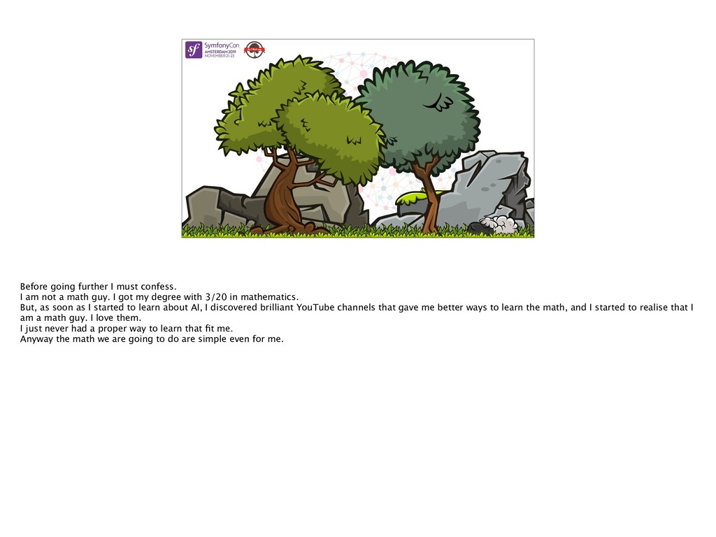
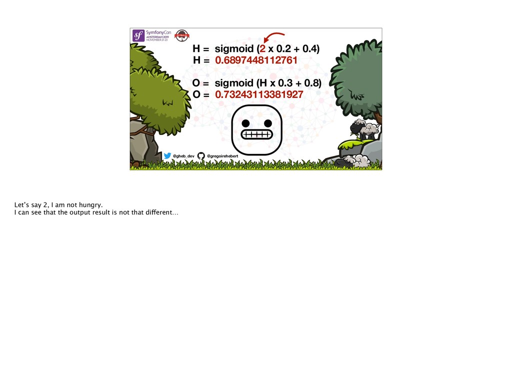
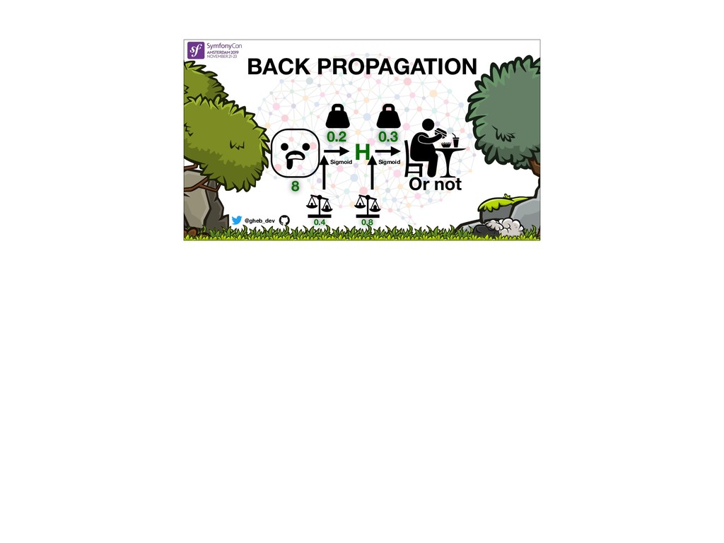
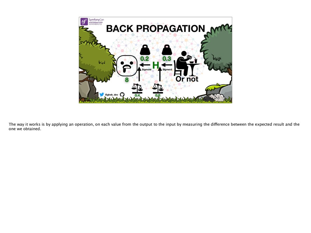
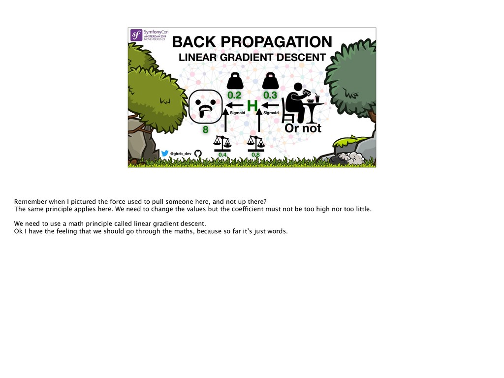
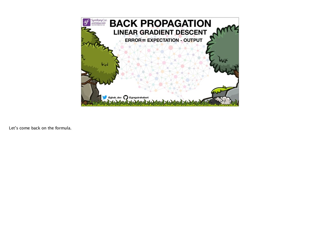
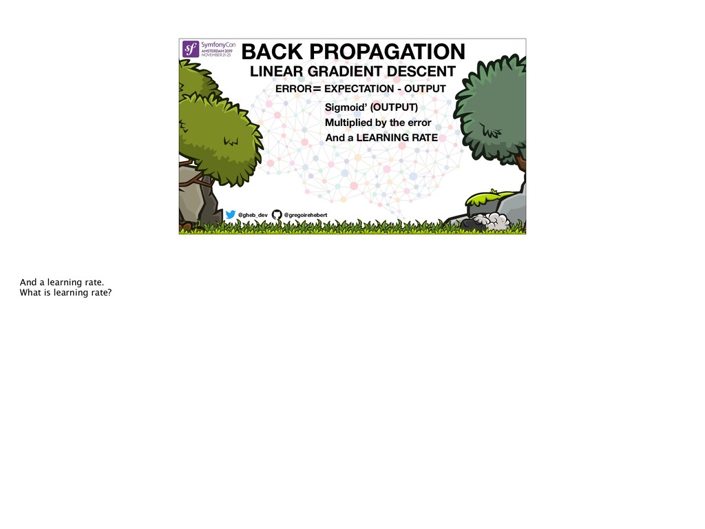
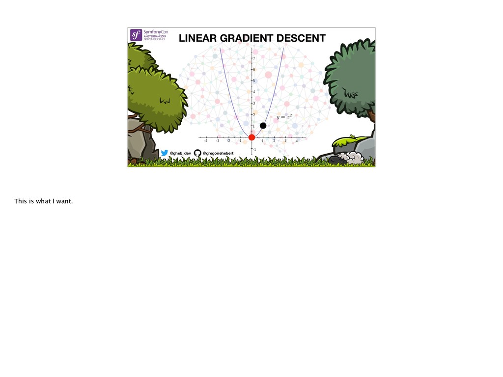
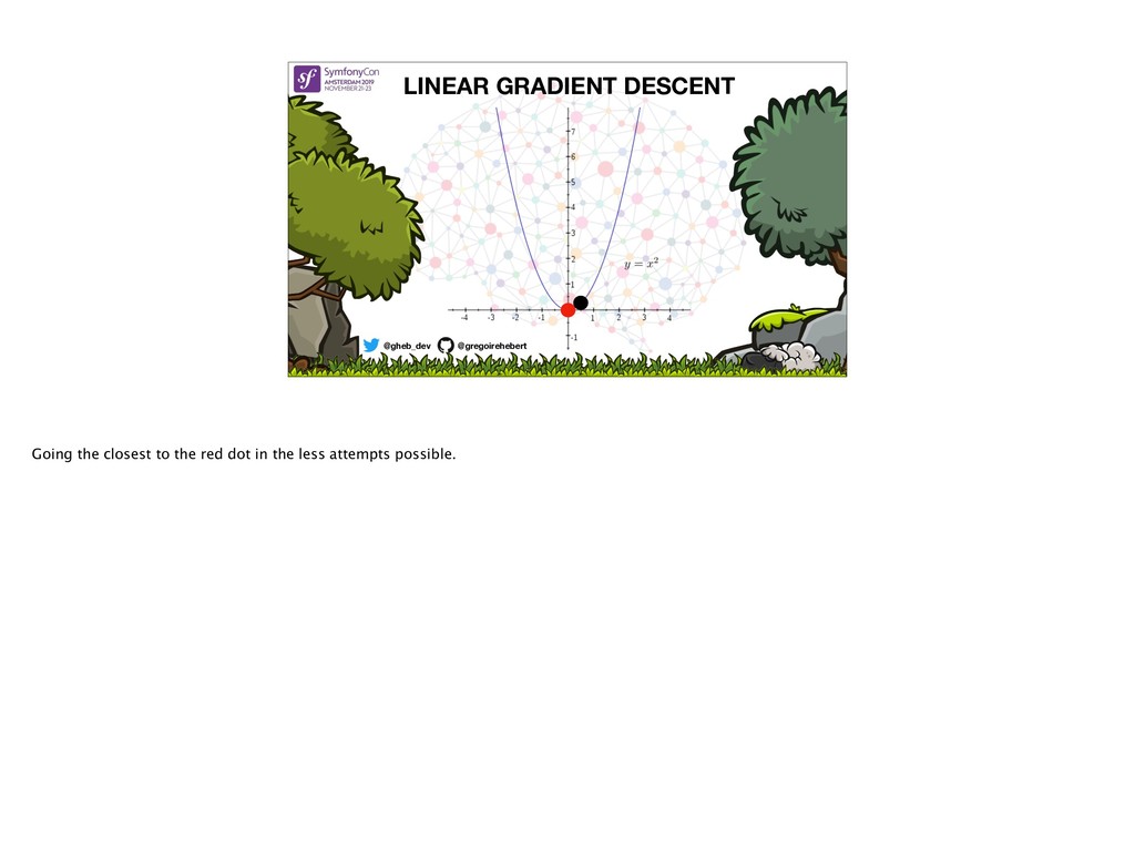
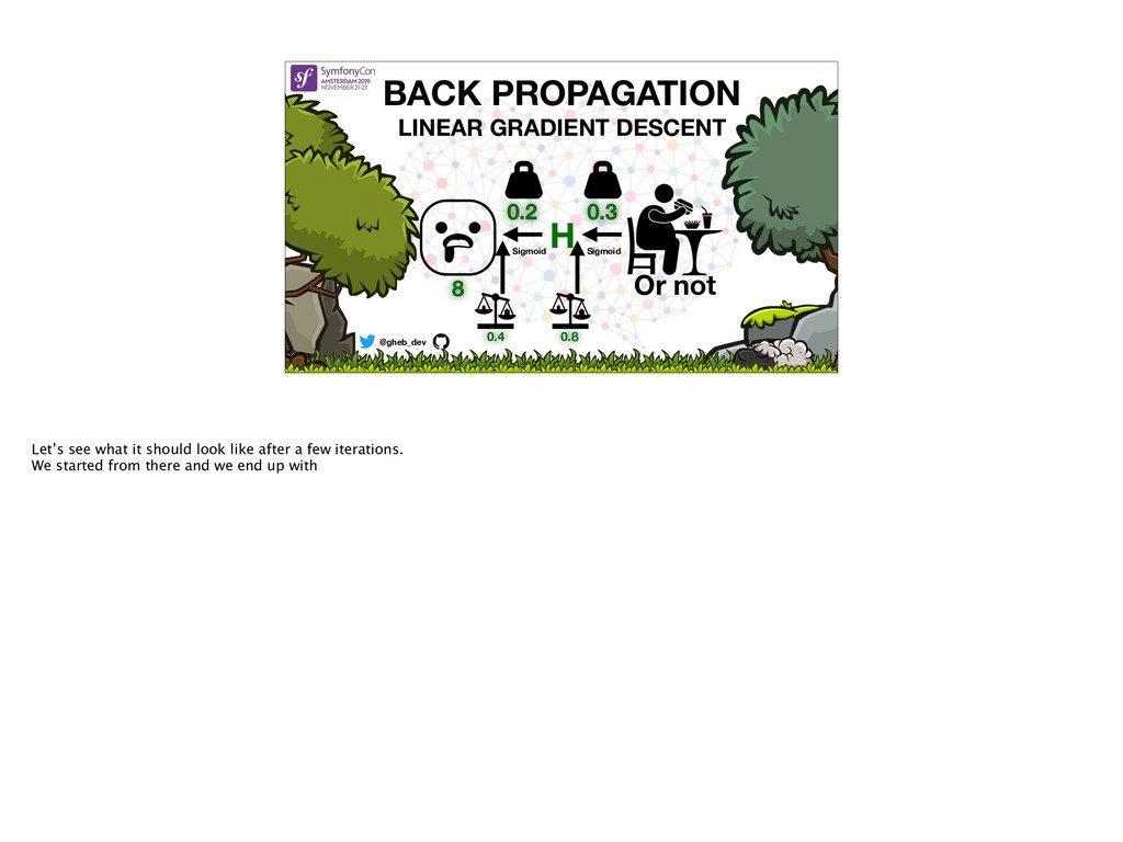
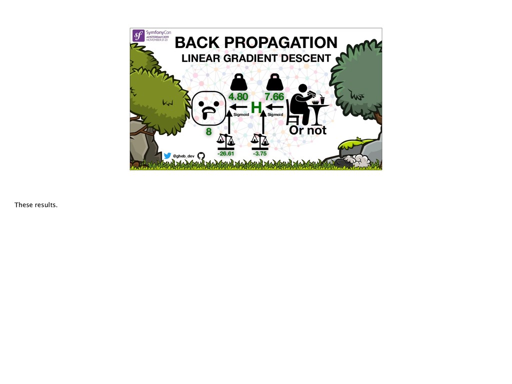
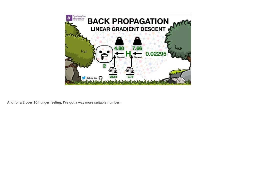
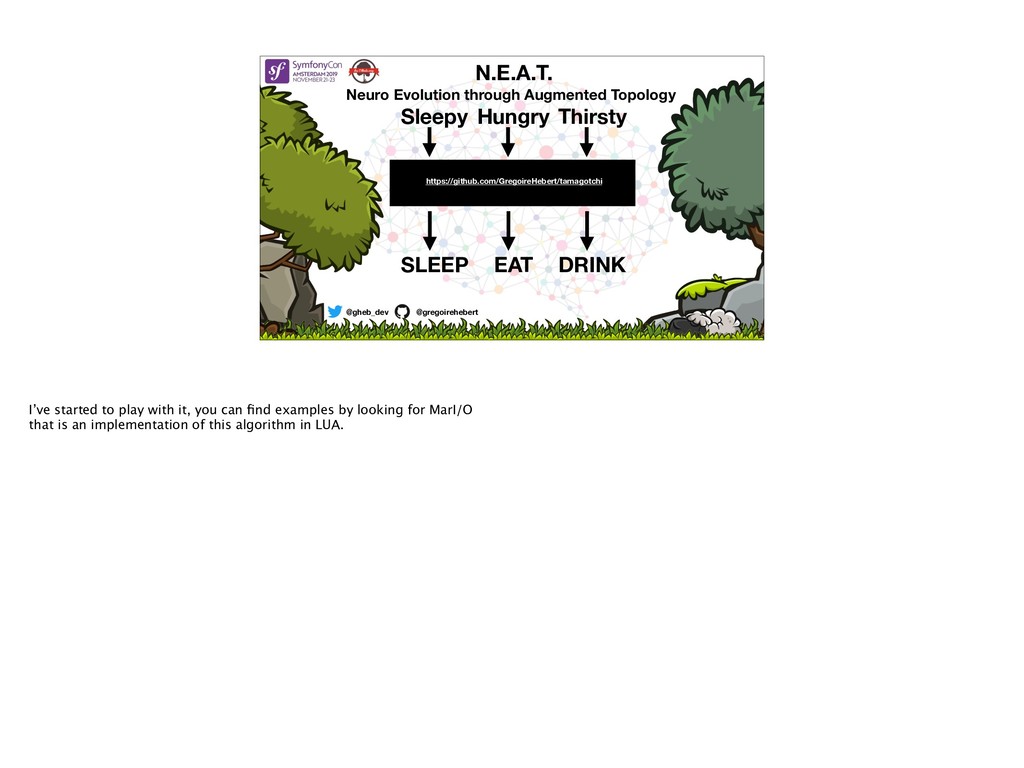
You've heard about AI for some time. But it remains obscure for you. How does it work, what is behind this word? If for you, reading white papers or doctoral papers is not your thing, that the Tensorflow doc is just a big pile of words for you, and if you've seen unclear presentations using the same vocabulary without really giving you an idea of how it works and how to implement an AI at home... This presentation is for you. At its end, you will be able to play with an AI, simple, but that will serve as a gateway to the beautiful world of machine-learning.
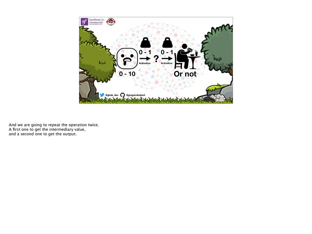
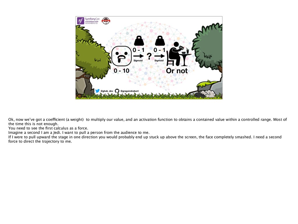
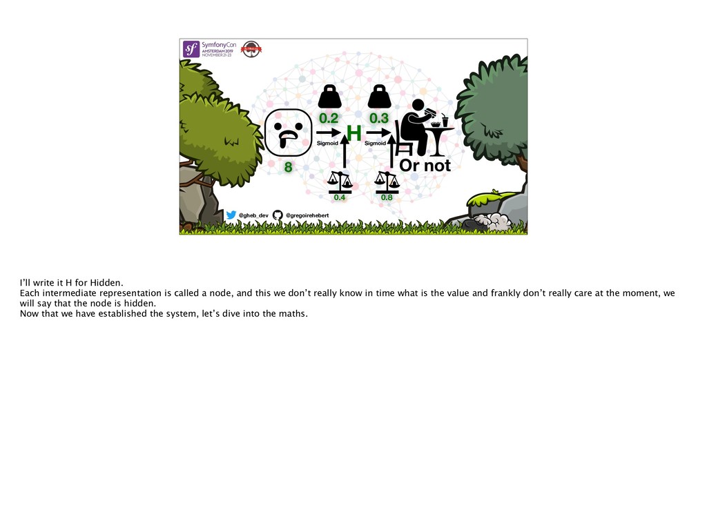
Grégoire Hébert

November 22, 2019
Tweet

More Decks by Grégoire Hébert

Other Decks in Programming

Transcript

  1. AN AI

    NEAT PLUS ULTRA

    View Slide

  2. AN AI

    NEAT PLUS ULTRA
    Good Afternoon everyone.
    I am thrilled to be here with you on stage!

    View Slide

  3. Grégoire Hébert
    Senior Developper — Trainer — Lecturer @ Les-Tilleuls.coop
    @gheb_dev
    @gregoirehebert
    UNE IA

    NEAT PLUS ULTRA
    Let me introduce myself :)

    My name is Grégoire Hébert, I am a senior developer, lecturer and speaker at Les-Tilleuls.coop .

    If you can’t pronounce it properly come at our booth, we’ll teach you :)


    View Slide

  4. @gheb_dev @gregoirehebert

    View Slide

  5. @gheb_dev @gregoirehebert
    Machine Learning
    Image Recognition
    Language Processing Autonomous Vehicules
    Medical Diagnostics
    Robotic
    Recommender Systems
    We are going to spend 40 minutes together, and the subject is the machine learning.

    Who, in this room, never worked with artificial intelligence before? Raise your hand.
    For all the others, what I am about to say may sound trivial, or simplistic, but the goal here is to set a start.

    Because YES. Doing research about Machine learning is not, something trivial.
    Machine learning is a subpart of the AI field, but is also part of the others.
    Without mentioning them, I showed some fields of usage, we are going to focus on things the we want to set autonomous. Now, How complex can be an
    AI? Does an AI has to be all powerful?

    Of course not,
    we’ve got multiple levels of complexity.

    Starting from

    View Slide

  6. @gheb_dev @gregoirehebert

    View Slide

  7. @gheb_dev @gregoirehebert
    REACTIVE MACHINES (Scenarii reactive)
    Reactive machine, this is the kind of AI, we have in video games.

    View Slide

  8. @gheb_dev @gregoirehebert
    REACTIVE MACHINES (Senarii reactive)
    LIMITED MEMORY (Environment reactive)
    Limited Memory, where we begin to act according to time, location, extra knowledge surrounding you.

    For instance, my car gps knows I am leaving the office, it’s 6p.m. it shows me every known restaurant on my way home.

    View Slide

  9. @gheb_dev @gregoirehebert
    REACTIVE MACHINES (Senarii reactive)
    LIMITED MEMORY (Environment reactive)
    THEORY OF MIND (People awareness)
    For the Theory of mind, it’s not just a blind guess anymore.
    The AI knows me ! I had a harsh day, It’ll show my favourite comforting restaurant..

    . Mc Donald, KFC… and a little padthai restaurant.

    View Slide

  10. @gheb_dev @gregoirehebert
    REACTIVE MACHINES (Senarii reactive)
    LIMITED MEMORY (Environment reactive)
    THEORY OF MIND (People awareness)
    SELF AWARE
    Self aware !! Beware ! It start to rule the world !

    View Slide

  11. SELF AWARE
    @gheb_dev @gregoirehebert
    REACTIVE MACHINES (Senarii reactive)
    LIMITED MEMORY (Environment reactive)
    THEORY OF MIND (People awareness)

    View Slide

  12. @gheb_dev @gregoirehebert
    REACTIVE MACHINES (Senarii reactive)
    Ok before that, we need to grasp the subtleties of the first level, ReactiveMachine.

    And don’t mistaken it’s simplicity for a lack of capabilities.
    The goal now is, together, see how each one of you could leave this room and be able to write down a simple AI.
    And then, be drown to the abyss of machine learning, even grow a passion to it :)

    View Slide

  13. @gheb_dev @gregoirehebert
    INPUT
    Alright, everything start from an input.

    An input can be a number, a set of numbers, an image, a string.
    Well, If I want to treat everything the same way, I’ll need to normalise that input.

    For a picture of my cat, I need to transform that jpeg file into a matrix of values, each one between 0 and 255 of white
    0 and 255 of red, of green and of blue. For each type of data I need to normalise it’s representation into something the system can read and exploit. The
    larger is the set, the better is the result.

    View Slide

  14. @gheb_dev @gregoirehebert
    INPUT
    ?
    That input will be computed into a value.

    At the moment we don’t know how.

    View Slide

  15. @gheb_dev @gregoirehebert
    INPUT
    ?
    OUTPUT
    And that value, will in the end be computed into a result.

    This result is the output we expect, the answer if you will.

    View Slide

  16. @gheb_dev @gregoirehebert
    INPUT ? OUTPUT
    PERCEPTRON
    Well this simplest representation is called a perceptron.
    Let’s put that into something representative shall we?

    View Slide

  17. @gheb_dev @gregoirehebert
    ?
    Let’s say, according to my hunger, the machine should decide if I shall eat.

    View Slide

  18. @gheb_dev @gregoirehebert
    ?
    Or not
    Or not.

    View Slide

  19. @gheb_dev @gregoirehebert
    ?
    Or not
    0 - 10
    To decide I need to normalise my stomach emptiness,
    0 : I am not hungry
    10: I am starving

    View Slide

  20. @gheb_dev @gregoirehebert
    ?
    Or not
    0 - 10
    0 - 1
    Activation
    To get to the intermediate value I will use a weight.

    This weight is at start a random value between 0 and 1.

    This is arbitrary it could be between 1 and 10 or 100. It’s up to you.

    How to chose then, it’s by experience. By running through a lot of dataset, you start having a spider sense about where the final value could be.

    View Slide

  21. @gheb_dev @gregoirehebert
    ?
    Or not
    0 - 10
    0 - 1
    Activation
    We are going then to use the result of the weight multiplied by the input 

    through an activation function.

    An activation function will help us to control the transformation of the input value into an output value according to their behaviour.

    View Slide

  22. @gheb_dev @gregoirehebert
    0 - 10
    ?
    Or not
    0 - 1 0 - 1
    Activation Activation

    View Slide

  23. @gheb_dev @gregoirehebert
    What is an activation function? It’s a a function,

    A mathematical function. Well not really one function.

    There are few functions that are useful as an activation function.

    View Slide

  24. @gheb_dev @gregoirehebert
    Binary Step
    You’ve got the Binary step.

    View Slide

  25. @gheb_dev @gregoirehebert
    Binary Step
    The easiest, according to the input value it will return a 0, or a 1.

    View Slide

  26. @gheb_dev @gregoirehebert
    Binary Step
    Gaussian
    The gaussian

    View Slide

  27. @gheb_dev @gregoirehebert
    Binary Step
    Gaussian
    This one, if you do statistics you know it well :) 

    It’s the same curve that represent the normal randomness distribution.

    View Slide

  28. @gheb_dev @gregoirehebert
    Binary Step
    Gaussian
    Hyperbolic Tangent

    View Slide

  29. @gheb_dev @gregoirehebert
    Binary Step
    Gaussian
    Hyperbolic Tangent
    TanH

    View Slide

  30. @gheb_dev @gregoirehebert
    Binary Step
    Gaussian
    Hyperbolic Tangent
    Parametric Rectified Linear Unit
    Relu

    View Slide

  31. @gheb_dev @gregoirehebert
    Binary Step
    Gaussian
    Hyperbolic Tangent
    Parametric Rectified Linear Unit
    Start a 0, and tends to infinite

    View Slide

  32. @gheb_dev @gregoirehebert
    Binary Step
    Gaussian
    Hyperbolic Tangent
    Parametric Rectified Linear Unit
    Sigmoid
    Sigmoid

    View Slide

  33. @gheb_dev @gregoirehebert
    Binary Step
    Gaussian
    Hyperbolic Tangent
    Parametric Rectified Linear Unit
    Sigmoid
    Tends toward 0 and 1 but never touches them.

    View Slide

  34. @gheb_dev @gregoirehebert
    Binary Step
    Gaussian
    Hyperbolic Tangent
    Parametric Rectified Linear Unit
    Sigmoid
    Thresholded Rectified Linear Unit

    View Slide

  35. @gheb_dev @gregoirehebert
    Binary Step
    Gaussian
    Hyperbolic Tangent
    Parametric Rectified Linear Unit
    Sigmoid
    Thresholded Rectified Linear Unit
    Like relu but with a threshold.

    View Slide

  36. @gheb_dev @gregoirehebert
    Binary Step
    Gaussian
    Hyperbolic Tangent
    Parametric Rectified Linear Unit
    Sigmoid
    Thresholded Rectified Linear Unit
    The most common one is Sigmoid, that’s the one we are going to use today.

    View Slide

  37. @gheb_dev @gregoirehebert
    Sigmoid

    View Slide

  38. 0 - 10
    ?
    0 - 1 0 - 1
    Activation Activation

    View Slide

  39. ?
    Or not
    0 - 10
    0 - 1 0 - 1
    Activation Activation
    @gheb_dev @gregoirehebert
    And we are going to repeat the operation twice.

    A first one to get the intermediary value, 

    and a second one to get the output.

    View Slide

  40. @gheb_dev @gregoirehebert
    ?
    Or not
    0 - 10
    0 - 1 0 - 1
    Sigmoid Sigmoid
    Ok, now we’ve got a coefficient (a weight) to multiply our value, and an activation function to obtains a contained value within a controlled range. Most of
    the time this is not enough.
    You need to see the first calculus as a force.

    Imagine a second I am a Jedi. I want to pull a person from the audience to me.

    If I were to pull upward the stage in one direction you would probably end up stuck up above the screen, the face completely smashed. I need a second
    force to direct the trajectory to me.

    View Slide

  41. ?
    Or not
    0 - 10
    0 - 1 0 - 1
    Sigmoid Sigmoid
    @gheb_dev @gregoirehebert
    I need a bias to apply to the value.

    View Slide

  42. ?
    Or not
    0 - 10
    0 - 1 0 - 1
    Sigmoid Sigmoid
    @gheb_dev @gregoirehebert
    Bias Bias
    This bias will be a factor, another simple addition to run.
    Their value, at start, are, like the weights, chosen at random, between 0 and 1.

    As before it could be to 10 or 100.

    Let’s change that into possible numbers for the example.

    View Slide

  43. ?
    Or not
    8
    0.2 0.3
    Sigmoid Sigmoid
    @gheb_dev @gregoirehebert
    0.4 0.8
    In this situation I am hungry.

    0.2 and 0.3 are the weight and 0.4 and 0.8 respectively the biases.
    Note that I did not named the value in between the input and the output.
    That intermediate representation.

    View Slide

  44. H
    Or not
    8
    0.2 0.3
    Sigmoid Sigmoid
    @gheb_dev @gregoirehebert
    0.4 0.8
    I’ll write it H for Hidden.

    Each intermediate representation is called a node, and this we don’t really know in time what is the value and frankly don’t really care at the moment, we
    will say that the node is hidden.
    Now that we have established the system, let’s dive into the maths.

    View Slide

  45. 0 - 10
    ?
    0 - 1 0 - 1
    Activation Activation
    Before going further I must confess.

    I am not a math guy. I got my degree with 3/20 in mathematics.

    But, as soon as I started to learn about AI, I discovered brilliant YouTube channels that gave me better ways to learn the math, and I started to realise that I
    am a math guy. I love them.

    I just never had a proper way to learn that fit me.

    Anyway the math we are going to do are simple even for me.

    View Slide

  46. @gheb_dev @gregoirehebert
    H = sigmoid (Input x weight + bias)
    To get the hidden value, 

    We need calculate the input multiplied by the weight plus the bias.

    the result will be passed into sigmoid.

    View Slide

  47. @gheb_dev @gregoirehebert
    H = sigmoid (8 x 0.2 + 0.4)
    With our example numbers this gives us sigmoid(8 x 0.2 + 0.4)

    View Slide

  48. @gheb_dev @gregoirehebert
    H = sigmoid (8 x 0.2 + 0.4)
    H = 0.88078707797788
    The result is 0.8807…
    Is it good? We don’t know. We need to do every operation.

    View Slide

  49. @gheb_dev @gregoirehebert
    H = sigmoid (8 x 0.2 + 0.4)
    H = 0.88078707797788
    O = sigmoid (H x W + B)
    Now the output is the sigmoid(H x W + B)

    View Slide

  50. @gheb_dev @gregoirehebert
    H = sigmoid (8 x 0.2 + 0.4)
    H = 0.88078707797788
    O = sigmoid (H x 0.3 + 0.8)
    With our example value it’s sigmoid (0.8807 x 0.3 + 0.8)

    View Slide

  51. @gheb_dev @gregoirehebert
    H = sigmoid (8 x 0.2 + 0.4)
    H = 0.88078707797788
    O = sigmoid (H x 0.3 + 0.8)
    O = 0.74349981350761
    It gives us 0.74.
    Let’s agree that over 0.5 I eat, and under, I don’t.

    View Slide

  52. @gheb_dev @gregoirehebert
    H = sigmoid (8 x 0.2 + 0.4)
    H = 0.88078707797788
    O = sigmoid (H x 0.3 + 0.8)
    O = 0.74349981350761
    I was hungry, And I eat :D

    View Slide

  53. @gheb_dev @gregoirehebert
    H = sigmoid (8 x 0.2 + 0.4)
    H = 0.88078707797788
    O = sigmoid (H x 0.3 + 0.8)
    O = 0.74349981350761
    Is it good, first run?
    To know, I need to run all the math with a lower input.

    View Slide

  54. @gheb_dev @gregoirehebert
    H = sigmoid (2 x 0.2 + 0.4)
    H = 0.6897448112761
    O = sigmoid (H x 0.3 + 0.8)
    O = 0.73243113381927
    Let’s say 2, I am not hungry.

    I can see that the output result is not that different…

    View Slide

  55. @gheb_dev @gregoirehebert
    H = sigmoid (2 x 0.2 + 0.4)
    H = 0.6897448112761
    O = sigmoid (H x 0.3 + 0.8)
    O = 0.73243113381927
    I ate too much. I would have died like a filleted goose.

    We need to fix the weights and biases until the numbers are right.

    View Slide

  56. H = sigmoid (2 x 0.2 + 0.4)
    H = 0.6897448112761
    O = sigmoid (H x 0.3 + 0.8)
    O = 0.73243113381927
    @gheb_dev @gregoirehebert
    TRAINING
    We need to train our system.

    View Slide

  57. @gheb_dev @gregoirehebert
    H = sigmoid (2 x 0.2 + 0.4)
    H = 0.6897448112761
    O = sigmoid (H x 0.3 + 0.8)
    O = 0.73243113381927

    View Slide

  58. H
    Or not
    8
    0.2 0.3
    Sigmoid Sigmoid
    @gheb_dev @gregoirehebert
    0.4 0.8
    BACK PROPAGATION
    The training system I am going to show you is called back propagation.
    It’s purpose it to correct iteration after iteration each value of the weights and biases until the result satisfy our goal.

    View Slide

  59. H
    Or not
    8
    0.2 0.3
    Sigmoid Sigmoid
    @gheb_dev 0.4 0.8
    BACK PROPAGATION

    View Slide

  60. H
    Or not
    8
    0.2 0.3
    Sigmoid Sigmoid
    @gheb_dev 0.4 0.8
    BACK PROPAGATION
    The way it works is by applying an operation, on each value from the output to the input by measuring the difference between the expected result and the
    one we obtained.

    View Slide

  61. H
    Or not
    8
    0.2 0.3
    Sigmoid Sigmoid
    @gheb_dev 0.4 0.8
    BACK PROPAGATION
    LINEAR GRADIENT DESCENT
    Remember when I pictured the force used to pull someone here, and not up there?

    The same principle applies here. We need to change the values but the coefficient must not be too high nor too little.
    We need to use a math principle called linear gradient descent.

    Ok I have the feeling that we should go through the maths, because so far it’s just words.


    View Slide

  62. @gheb_dev @gregoirehebert
    BACK PROPAGATION
    LINEAR GRADIENT DESCENT
    ERROR
    ok, we need to get the error. So the difference between the result and what’s expected.

    View Slide

  63. @gheb_dev @gregoirehebert
    BACK PROPAGATION
    LINEAR GRADIENT DESCENT
    It can be for a single point, or the median to a dataset.

    View Slide

  64. @gheb_dev @gregoirehebert
    BACK PROPAGATION
    LINEAR GRADIENT DESCENT
    ERROR EXPECTATION - OUTPUT
    =
    Grab and subtract the two values.
    You’ve got the error.

    If I were to apply the difference directly into each value, the result might not be the one we expect.

    View Slide

  65. @gheb_dev @gregoirehebert
    BACK PROPAGATION
    LINEAR GRADIENT DESCENT
    ERROR EXPECTATION - OUTPUT
    =
    Let’s say we are in a world where friction does not exists.

    If I continuously apply the same force through time to the train…well

    View Slide

  66. @gheb_dev @gregoirehebert
    BACK PROPAGATION
    LINEAR GRADIENT DESCENT
    ERROR EXPECTATION - OUTPUT
    =

    View Slide

  67. @gheb_dev @gregoirehebert
    BACK PROPAGATION
    LINEAR GRADIENT DESCENT
    ERROR EXPECTATION - OUTPUT
    =
    Pfjrouu ! Yay roller coaster tycoon !

    View Slide

  68. @gheb_dev @gregoirehebert
    BACK PROPAGATION
    LINEAR GRADIENT DESCENT
    ERROR EXPECTATION - OUTPUT
    =
    We need to adjust a few things to get it working.

    View Slide

  69. @gheb_dev @gregoirehebert
    LINEAR GRADIENT DESCENT
    Imagine, we replace the rail track by this function representation.

    It’s quite similar. It’s a curve.

    My goal is to find the lowest position on the curve.

    View Slide

  70. @gheb_dev @gregoirehebert
    LINEAR GRADIENT DESCENT
    My starting point is arbitrary. 

    As a human with two properly working eyes, I can easily eyeball that I need to reduce the value.

    I am too far.

    But on a computer perspective how do I know that?

    View Slide

  71. @gheb_dev @gregoirehebert
    LINEAR GRADIENT DESCENT
    I need to find the slope.
    The slope will help us to find whether the next value increase or decrease, same for the previous value. So I can apply the right operation, should I go forth
    or go back.

    View Slide

  72. @gheb_dev @gregoirehebert
    LINEAR GRADIENT DESCENT
    Thanks to the slope I know I can go back.

    In math to get the function’s slope, we need to use what’s called its derivative.

    View Slide

  73. @gheb_dev @gregoirehebert
    LINEAR GRADIENT DESCENT
    The derivative or Slope


    For any function f, it’s derivative f’

    calculate the direction


    S >= 0 then you must increase the value

    S <= 0 then you must decrease the value
    The result of a derivative gives us the direction.

    If it’s over 0 we must increase the value, 

    under 0, we must decrease the value.
    Simple.

    View Slide

  74. @gheb_dev @gregoirehebert
    BACK PROPAGATION
    LINEAR GRADIENT DESCENT
    ERROR EXPECTATION - OUTPUT
    =
    Let’s come back on the formula.

    View Slide

  75. @gheb_dev @gregoirehebert
    BACK PROPAGATION
    LINEAR GRADIENT DESCENT
    ERROR EXPECTATION - OUTPUT
    =
    Sigmoid’ (OUTPUT)
    We apply the derivative of sigmoid, with the output as entry value.

    We’ve got a result which is?

    The slope, thank you to follow!

    View Slide

  76. @gheb_dev @gregoirehebert
    BACK PROPAGATION
    LINEAR GRADIENT DESCENT
    ERROR EXPECTATION - OUTPUT
    =
    Sigmoid’ (OUTPUT)
    Multiplied by the error
    We multiply this by the error.

    View Slide

  77. @gheb_dev @gregoirehebert
    BACK PROPAGATION
    LINEAR GRADIENT DESCENT
    ERROR EXPECTATION - OUTPUT
    =
    Sigmoid’ (OUTPUT)
    Multiplied by the error
    And a LEARNING RATE
    And a learning rate.

    What is learning rate?


    View Slide

  78. @gheb_dev @gregoirehebert
    LINEAR GRADIENT DESCENT
    This is what I want.

    View Slide

  79. @gheb_dev @gregoirehebert
    LINEAR GRADIENT DESCENT
    Going the closest to the red dot in the less attempts possible.

    View Slide

  80. @gheb_dev @gregoirehebert
    LINEAR GRADIENT DESCENT
    But according to the error, I have a chance to miss my point.

    Greater the error, bigger are the chances.

    View Slide

  81. @gheb_dev @gregoirehebert
    LINEAR GRADIENT DESCENT
    And I could swing around for a long moment.

    View Slide

  82. @gheb_dev @gregoirehebert
    LINEAR GRADIENT DESCENT

    View Slide

  83. @gheb_dev @gregoirehebert
    BACK PROPAGATION
    LINEAR GRADIENT DESCENT
    ERROR EXPECTATION - OUTPUT
    =
    Sigmoid’ (OUTPUT)
    Multiplied by the error
    And the LEARNING RATE
    I need a learning rate to temper this.

    Remember when I want to pull someone to stage, 

    I can prevent him to fly away to the sky, but if it is to break it’s spine to the floor…

    View Slide

  84. @gheb_dev @gregoirehebert
    BACK PROPAGATION
    LINEAR GRADIENT DESCENT
    ERROR EXPECTATION - OUTPUT
    =
    GRADIENT Sigmoid’ (OUTPUT)
    =
    Multiplied by the error
    And the LEARNING RATE
    We call the result of this formula the gradient. And this, is the coefficient we want to apply to our different weight and biases.

    But I must warn you.
    From the start we chose everything at random, expecting the values to be fixed through iterations. But the learning rate, you need to adjust it’s value. If it’s
    too high, you might never reach your goal by always passing by it but never stop close enough. And if it’s too small, You’ve got two problems coming, first
    one you will need way too many iterations to find the minimum value in the curb.
    The second one is you can get trapped in a valley. Let me show you this:

    View Slide

  85. @gheb_dev @gregoirehebert
    BACK PROPAGATION
    LINEAR GRADIENT DESCENT
    Beware of the local minimum
    If I am on the right part of the track, I’ll find a local minimum.

    But I can see that I am not it the lowest part of the track.

    This is when the human is useful. You know or have the feeling that it’s not right.

    In addition to say, here is the objective, you can adjust the learning rate so you can go over hills.

    This is where it can be complex and you might need to use more advanced systems.

    View Slide

  86. @gheb_dev @gregoirehebert
    BACK PROPAGATION
    LINEAR GRADIENT DESCENT
    ERROR EXPECTATION - OUTPUT
    =
    GRADIENT Sigmoid’ (OUTPUT)
    =
    Multiplied by the error
    And the LEARNING RATE
    ΔWeights GRADIENT x H
    =
    Alright, by multiplying the gradient to the hidden value, we’ve got the delta for the weights.

    View Slide

  87. H
    Or not
    8
    0.2 0.3
    Sigmoid Sigmoid
    @gheb_dev 0.4 0.8
    BACK PROPAGATION
    LINEAR GRADIENT DESCENT
    Remember pour little scheme ?
    We are going to go back for every single one of the four values.

    View Slide

  88. @gheb_dev @gregoirehebert
    BACK PROPAGATION
    LINEAR GRADIENT DESCENT
    ERROR EXPECTATION - OUTPUT
    =
    GRADIENT Sigmoid’ (OUTPUT)
    =
    Multiplied by the error
    And the LEARNING RATE
    ΔWeights GRADIENT x H
    =
    Weights ΔWeights + weights
    =
    The new weights values are now the delta (which might be negative) in addition to the previous weights values.

    View Slide

  89. @gheb_dev @gregoirehebert
    BACK PROPAGATION
    LINEAR GRADIENT DESCENT
    ERROR EXPECTATION - OUTPUT
    =
    GRADIENT Sigmoid’ (OUTPUT)
    =
    Multiplied by the error
    And the LEARNING RATE
    ΔWeights GRADIENT x H
    =
    Weights ΔWeights + weights
    =
    Bias Bias + GRADIENT
    =
    For the bias we don’t need that much of a difference, just adding the gradient do the trick.

    View Slide

  90. H
    Or not
    8
    0.2 0.3
    Sigmoid Sigmoid
    @gheb_dev
    0.4 0.8
    BACK PROPAGATION
    LINEAR GRADIENT DESCENT
    Let’s see what it should look like after a few iterations.
    We started from there and we end up with

    View Slide

  91. H
    Or not
    8
    4.80 7.66
    Sigmoid Sigmoid
    @gheb_dev
    -26.61 -3.75
    BACK PROPAGATION
    LINEAR GRADIENT DESCENT
    These results.

    View Slide

  92. H
    8
    4.80 7.66
    Sigmoid Sigmoid
    @gheb_dev
    -26.61 -3.75
    BACK PROPAGATION
    LINEAR GRADIENT DESCENT
    0.97988
    For this combination and a 8 over 10 hunger feeling, I got 0.97988 value.

    View Slide

  93. H
    4.80 7.66
    Sigmoid Sigmoid
    @gheb_dev
    -26.61 -3.75
    BACK PROPAGATION
    LINEAR GRADIENT DESCENT
    2
    0.02295
    And for a 2 over 10 hunger feeling, I’ve got a way more suitable number.

    View Slide

  94. H
    4.80 7.66
    Sigmoid Sigmoid
    @gheb_dev
    -26.61 -3.75
    BACK PROPAGATION
    LINEAR GRADIENT DESCENT
    2
    0.02295

    View Slide

  95. @gheb_dev @gregoirehebert
    CONGRATULATIONS !
    Congratulation ! You are already capable of creating a small yet powerful machine learning system.

    Who feels that building this kind of system is at reach now? Raise your hand.

    Alright for the others, let me show you, that you under-estimate yourselves.

    View Slide

  96. CONGRATULATIONS !
    Let’s play together :)
    https://github.com/GregoireHebert/nn/
    @gheb_dev @gregoirehebert
    You can grab the code and play with it at home.
    This is simple PHP, only one dependency to manipulate matrices of values, that’s it.
    We are in a symfony conference so I could not resist I made a small toy with this 

    and with 2 or 3 components from symfony I created a tamagotchi. An autonomous sheep :D

    It comes in an example branch, I installed a raspberry with an lcd screen, and asked a friend to print a box for me, that you have probably already seen on
    the booth.

    View Slide

  97. CONGRATULATIONS !
    Let’s play together :)
    @gheb_dev @gregoirehebert
    Now, that you have touched the most minimalistic system with the tip of the finger.

    What can we do to improve it and do things more complex?

    View Slide

  98. @gheb_dev @gregoirehebert
    Hungry
    EAT
    Well with a perceptron I can do that.

    View Slide

  99. @gheb_dev @gregoirehebert
    Hungry
    EAT
    But I can make it a little more complex, and have multiple hidden nodes each one with its own weights and biases. 

    Maybe for each node you can use a different activation function.

    View Slide

  100. @gheb_dev @gregoirehebert
    Hungry
    EAT
    MULTI LAYER PERCEPTRON
    Hungry
    EAT
    Hungry
    EAT
    We can multiply this horizontally and vertically into a multi layer perceptron

    View Slide

  101. @gheb_dev @gregoirehebert
    Hungry
    EAT
    MULTI LAYER PERCEPTRON
    Thirsty
    DRINK
    Sleepy
    SLEEP

    View Slide

  102. @gheb_dev @gregoirehebert
    Hungry
    EAT
    MULTI LAYER PERCEPTRON
    Thirsty
    DRINK
    Sleepy
    SLEEP
    Where each input has an impact on the others.

    Ok as far as we are now, we always have the control over the number of nodes and layers.
    What if….

    View Slide

  103. @gheb_dev @gregoirehebert
    Hungry
    EAT
    MULTI LAYER PERCEPTRON
    Thirsty
    DRINK
    Sleepy
    SLEEP
    We don’t.

    View Slide

  104. @gheb_dev @gregoirehebert
    Hungry
    EAT
    MULTI LAYER PERCEPTRON
    Thirsty
    DRINK
    Sleepy
    SLEEP
    What if, any decision his made randomly? Number of layers, nodes, weights, biases, their values.

    And to check over different configurations which one is the best, 


    Imagine we create hundreds of configurations randomly, put them all into competition and only keep the top 10. Then from the top ten we create a new
    set of 90 configurations with some slight mutations. And we go over and over. Until the results is satisfying.

    View Slide

  105. @gheb_dev @gregoirehebert
    Hungry
    EAT
    N.E.A.T.
    Thirsty
    DRINK
    Sleepy
    SLEEP
    Neuro Evolution through Augmented Topology
    This is called NEAT. Neuro evolution through augmented topology.

    This is really exciting !

    View Slide

  106. @gheb_dev @gregoirehebert
    Hungry
    EAT
    N.E.A.T.
    Thirsty
    DRINK
    Sleepy
    SLEEP
    Neuro Evolution through Augmented Topology
    https://github.com/GregoireHebert/tamagotchi
    I’ve started to play with it, you can find examples by looking for MarI/O

    that is an implementation of this algorithm in LUA.

    View Slide

  107. @gheb_dev @gregoirehebert

    View Slide

  108. @gheb_dev @gregoirehebert
    Going Further
    Data Normalization / Preparation


    Multiple Activation functions


    Mutations


    Unsupervised Learning

    So to summarise to go further, 

    You can dig into data normalisation and preparation, 

    multiple activation functions, applying mutations, and finish into the awesome vortex of unsupervised learning.

    View Slide

  109. @gheb_dev @gregoirehebert
    I don’t leave you without sources, Here are some youtube channels you can follow 


    View Slide

  110. @gheb_dev @gregoirehebert
    3blue1Brown which is an absolute goldmine for the math explanation of theorems and how neural networks works.

    The coding train is a teacher which has a tremendous amount of coding videos about machine learning. Even if in his case it’s more about drawings
    recognition and approximation, he has a full serie about the fundamentals.
    Computerphile is a concentrate of gold nuggets !

    View Slide

  111. @gheb_dev @gregoirehebert
    Something More PHP related, In PHP there is a huge library which is PHP-ML.

    And since we have access to foreign function interfaces (FFI) in php, you can now use TensorFlow in PHP. It’s experimental but.

    View Slide

  112. @gheb_dev @gregoirehebert
    There are two repositories, php-ffi and php-tensorflow.

    View Slide

  113. @gheb_dev @gregoirehebert

    View Slide

  114. @gheb_dev @gregoirehebert
    THANK YOU!
    Thank you so much that’s it for me :)
    I just have an ultimate question for you!

    View Slide

  115. @gheb_dev @gregoirehebert
    THANK YOU!
    How many sheeps did you see ?
    How many sheeps did you see during the presentation ? :)

    View Slide