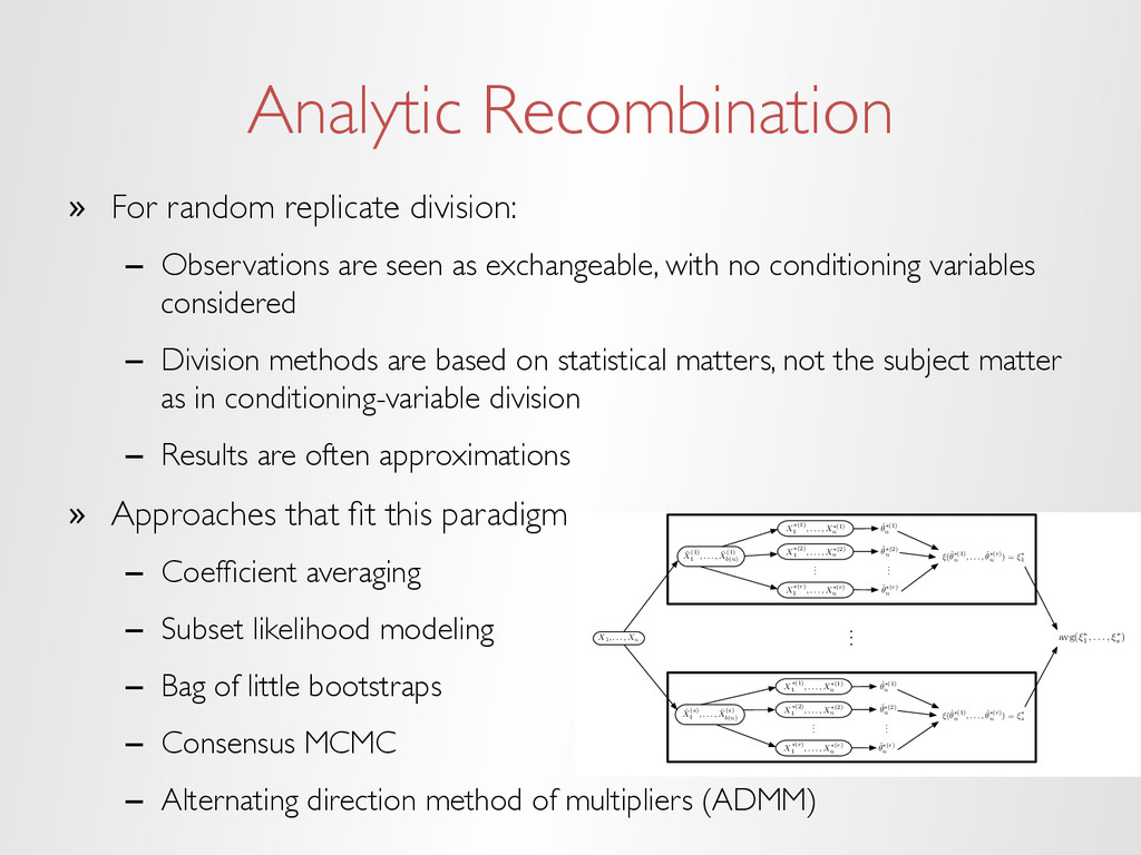
seen as exchangeable, with no conditioning variables considered – Division methods are based on statistical matters, not the subject matter as in conditioning-variable division – Results are often approximations » Approaches that fit this paradigm – Coefficient averaging – Subset likelihood modeling – Bag of little bootstraps – Consensus MCMC – Alternating direction method of multipliers (ADMM) Our Approach: BLB X1, . . . , Xn . . . . . . X⇤(1) 1 , . . . , X⇤(1) n X⇤(2) 1 , . . . , X⇤(2) n ˆ ✓⇤(1) n ˆ ✓⇤(2) n . . . . . . X⇤(1) 1 , . . . , X⇤(1) n X⇤(2) 1 , . . . , X⇤(2) n ˆ ✓⇤(1) n ˆ ✓⇤(2) n . . . ˇ X(1) 1 , . . . , ˇ X(1) b(n) avg(⇠⇤ 1 , . . . , ⇠⇤ s ) ˇ X(s) 1 , . . . , ˇ X(s) b(n) X⇤(r) 1 , . . . , X⇤(r) n X⇤(r) 1 , . . . , X⇤(r) n ˆ ✓⇤(r) n ˆ ✓⇤(r) n ⇠(ˆ ✓⇤(1) n , . . . , ˆ ✓⇤(r) n ) = ⇠⇤ 1 ⇠(ˆ ✓⇤(1) n , . . . , ˆ ✓⇤(r) n ) = ⇠⇤ s
![“If [you have no] concern about error bars, about heterogeneity,](https://files.speakerdeck.com/presentations/ef7b7f0616024d03ae8c8336659ab323/slide_4.jpg)
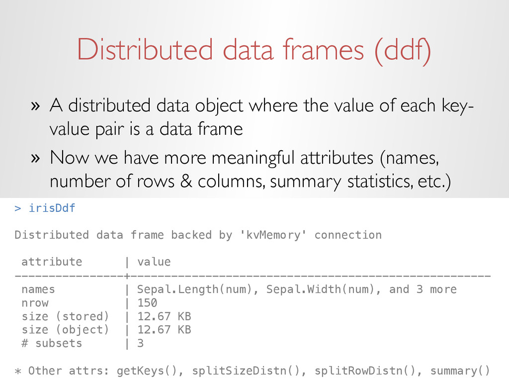
![[[1]]! $key! [1] "setosa"! ! $value! Sepal.Length Sepal.Width Petal.Length Petal.Width!](https://files.speakerdeck.com/presentations/ef7b7f0616024d03ae8c8336659ab323/slide_14.jpg)
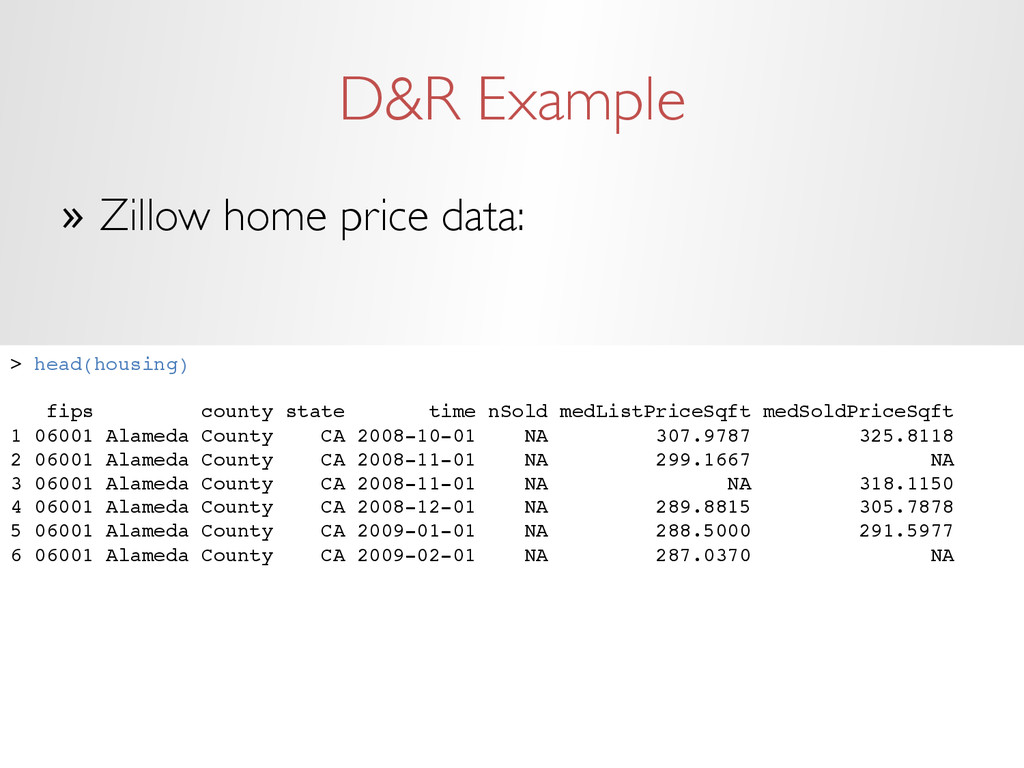
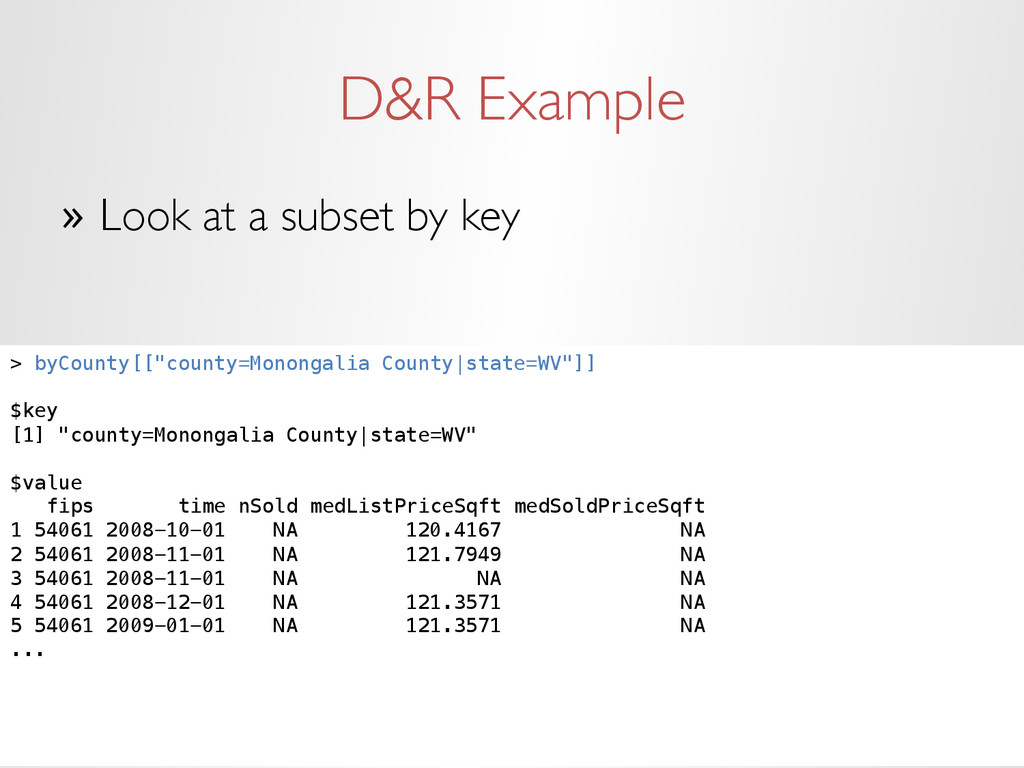
![D&R Example » Look at a subset > byCounty[[1]]! !](https://files.speakerdeck.com/presentations/ef7b7f0616024d03ae8c8336659ab323/slide_31.jpg)