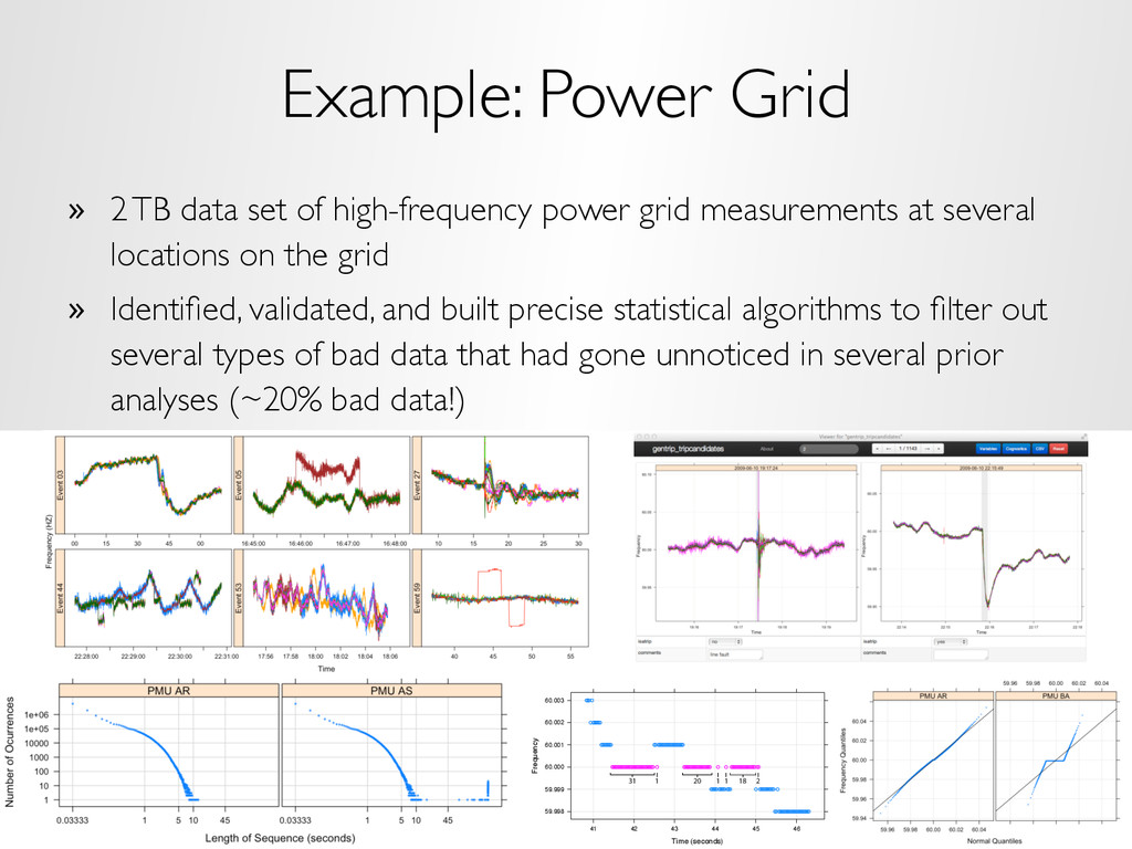
power grid measurements at several locations on the grid » Identified, validated, and built precise statistical algorithms to filter out several types of bad data that had gone unnoticed in several prior analyses (~20% bad data!) Time (seconds) Frequency 59.998 59.999 60.000 60.001 60.002 60.003 41 42 43 44 45 46 31 1 20 1 1 18 2
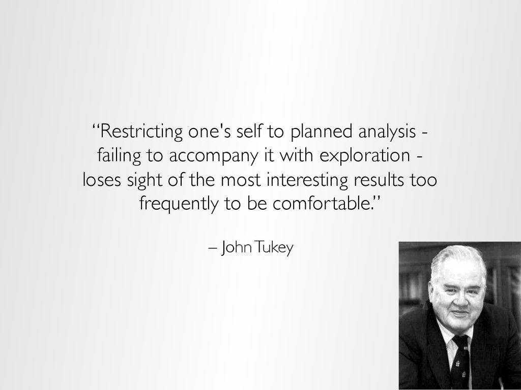
about noisy data, about the sampling pattern, about all the kinds of things that you have to be serious about if you’re a statistician – then … there’s a good chance that you will occasionally solve some real interesting problems. But you will occasionally have some disastrously bad decisions. And you won’t know the difference a priori. You will just produce these outputs and hope for the best.” – Michael Jordan
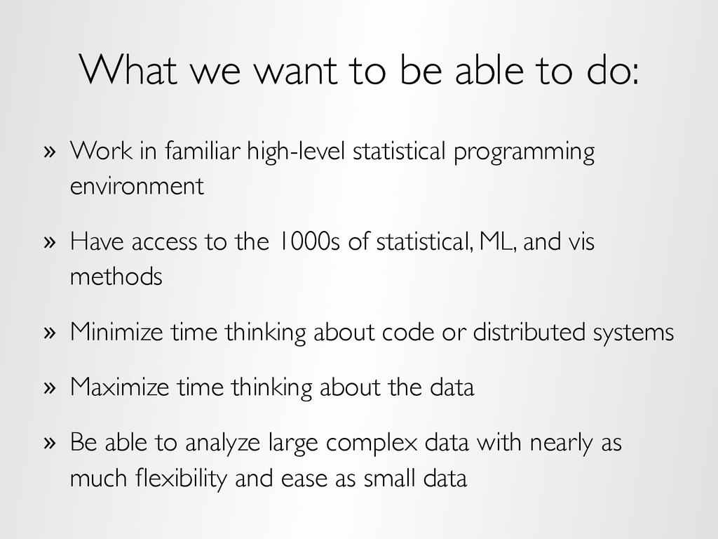
in familiar high-level statistical programming environment » Have access to the 1000s of statistical, ML, and vis methods » Minimize time thinking about code or distributed systems » Maximize time thinking about the data » Be able to analyze large complex data with nearly as much flexibility and ease as small data
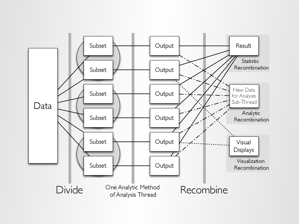
divisions of the data – analytic or visual methods are applied independently to each subset of the divided data in embarrassingly parallel fashion – Results are recombined to yield a statistically valid D&R result for the analytic method » D&R is not the same as MapReduce (but makes heavy use of it)
Output Output Output Output One Analytic Method of Analysis Thread Recombine Result Statistic Recombination New Data for Analysis Sub-Thread Analytic Recombination Visual Displays Visualization Recombination
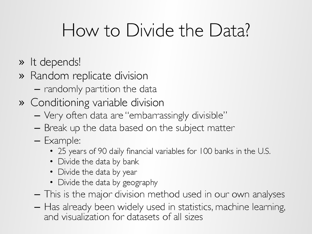
replicate division – randomly partition the data » Conditioning variable division – Very often data are “embarrassingly divisible” – Break up the data based on the subject matter – Example: • 25 years of 90 daily financial variables for 100 banks in the U.S. • Divide the data by bank • Divide the data by year • Divide the data by geography – This is the major division method used in our own analyses – Has already been widely used in statistics, machine learning, and visualization for datasets of all sizes
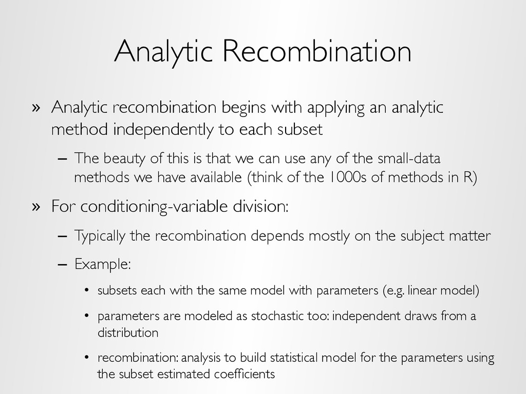
method independently to each subset – The beauty of this is that we can use any of the small-data methods we have available (think of the 1000s of methods in R) » For conditioning-variable division: – Typically the recombination depends mostly on the subject matter – Example: • subsets each with the same model with parameters (e.g. linear model) • parameters are modeled as stochastic too: independent draws from a distribution • recombination: analysis to build statistical model for the parameters using the subset estimated coefficients
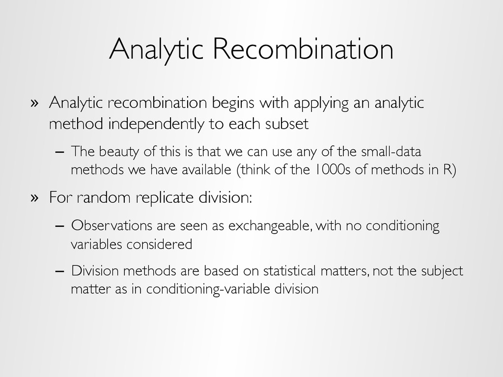
method independently to each subset – The beauty of this is that we can use any of the small-data methods we have available (think of the 1000s of methods in R) » For random replicate division: – Observations are seen as exchangeable, with no conditioning variables considered – Division methods are based on statistical matters, not the subject matter as in conditioning-variable division
= X + ✏ Linear model: ˆ = r X s=1 X0 s Xs ! 1 r X s=1 X0 s Ys Entire-data least squares estimate: ¨ = 1 r r X s=1 (X0 s Xs) 1X0 s Ys D&R approximation: ¨ ⇡ ˆ Under certain conditions, we can show: Partition into random subsets: 2 6 6 6 4 Y1 Y2 . . . Yr 3 7 7 7 5 = 2 6 6 6 4 X1 X2 . . . Xr 3 7 7 7 5 + 2 6 6 6 4 ✏1 ✏ . . . ✏ 3 7 7 7 5
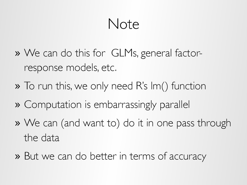
response models, etc. » To run this, we only need R’s lm() function » Computation is embarrassingly parallel » We can (and want to) do it in one pass through the data » But we can do better in terms of accuracy
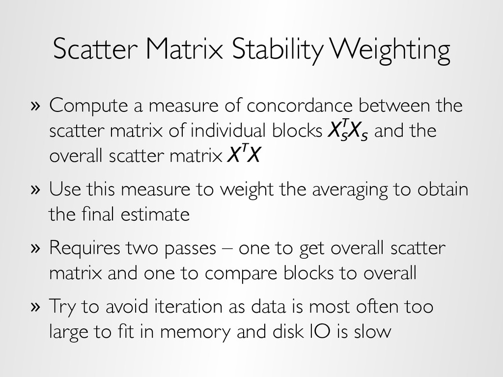
between the scatter matrix of individual blocks XT S X S and the overall scatter matrix XTX » Use this measure to weight the averaging to obtain the final estimate » Requires two passes – one to get overall scatter matrix and one to compare blocks to overall » Try to avoid iteration as data is most often too large to fit in memory and disk IO is slow
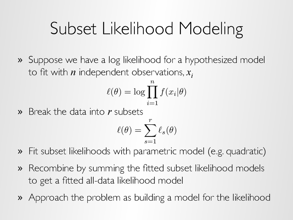
for a hypothesized model to fit with n independent observations, xi » Break the data into r subsets » Fit subset likelihoods with parametric model (e.g. quadratic) » Recombine by summing the fitted subset likelihood models to get a fitted all-data likelihood model » Approach the problem as building a model for the likelihood `(✓) = log n Y i=1 f(xi | ✓) `(✓) = r X s=1 `s(✓)
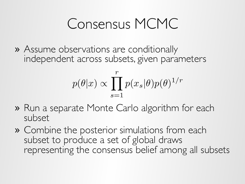
given parameters » Run a separate Monte Carlo algorithm for each subset » Combine the posterior simulations from each subset to produce a set of global draws representing the consensus belief among all subsets p ( ✓ | x ) / r Y s=1 p ( xs | ✓ ) p ( ✓ )1/r
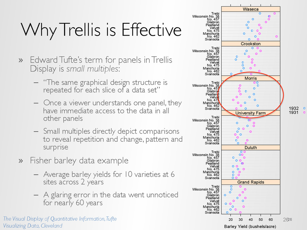
in Trellis Display is small multiples: – “The same graphical design structure is repeated for each slice of a data set” – Once a viewer understands one panel, they have immediate access to the data in all other panels – Small multiples directly depict comparisons to reveal repetition and change, pattern and surprise » Fisher barley data example – Average barley yields for 10 varieties at 6 sites across 2 years – A glaring error in the data went unnoticed for nearly 60 years 26 26 Barley Yield (bushels/acre) Svansota No. 462 Manchuria No. 475 Velvet Peatland Glabron No. 457 Wisconsin No. 38 Trebi 20 30 40 50 60 Grand Rapids Svansota No. 462 Manchuria No. 475 Velvet Peatland Glabron No. 457 Wisconsin No. 38 Trebi Duluth Svansota No. 462 Manchuria No. 475 Velvet Peatland Glabron No. 457 Wisconsin No. 38 Trebi University Farm Svansota No. 462 Manchuria No. 475 Velvet Peatland Glabron No. 457 Wisconsin No. 38 Trebi Morris Svansota No. 462 Manchuria No. 475 Velvet Peatland Glabron No. 457 Wisconsin No. 38 Trebi Crookston Svansota No. 462 Manchuria No. 475 Velvet Peatland Glabron No. 457 Wisconsin No. 38 Trebi Waseca 1932 1931 The Visual Display of Quantitative Information, Tufte Visualizing Data, Cleveland
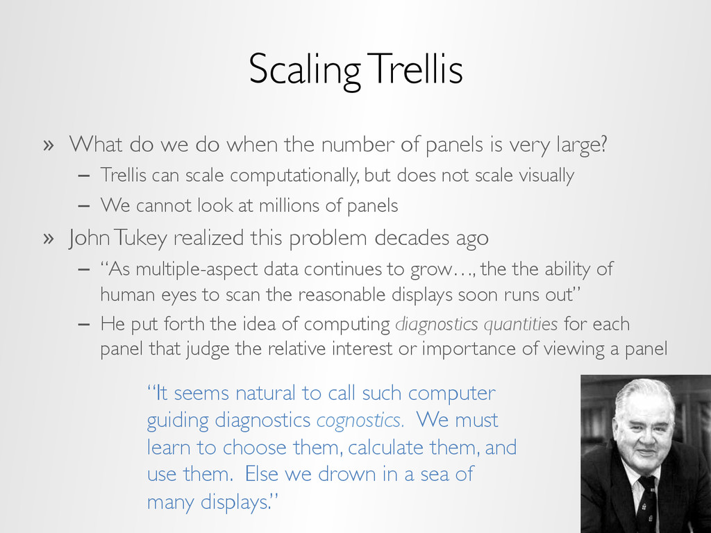
of panels is very large? – Trellis can scale computationally, but does not scale visually – We cannot look at millions of panels » John Tukey realized this problem decades ago – “As multiple-aspect data continues to grow…, the the ability of human eyes to scan the reasonable displays soon runs out” – He put forth the idea of computing diagnostics quantities for each panel that judge the relative interest or importance of viewing a panel “It seems natural to call such computer guiding diagnostics cognostics. We must learn to choose them, calculate them, and use them. Else we drown in a sea of many displays.”
a set of cognostics, metrics that identify an attribute of interest in the subset » Recombine visually by sampling, sorting, or filtering subsets based on the cognostics » Cognostics are computed for all subsets » Panels are not
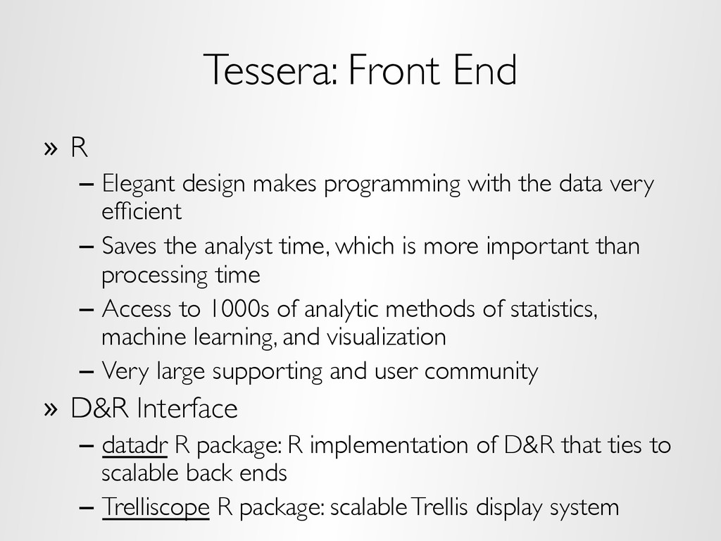
with the data very efficient – Saves the analyst time, which is more important than processing time – Access to 1000s of analytic methods of statistics, machine learning, and visualization – Very large supporting and user community » D&R Interface – datadr R package: R implementation of D&R that ties to scalable back ends – Trelliscope R package: scalable Trellis display system
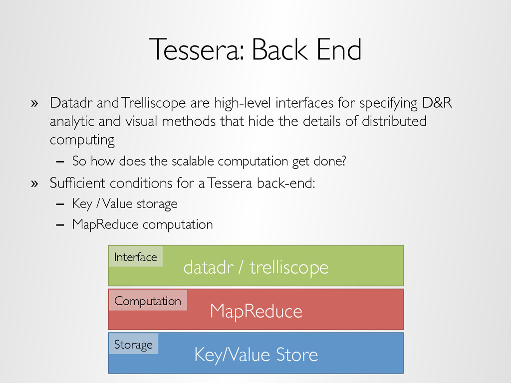
for specifying D&R analytic and visual methods that hide the details of distributed computing – So how does the scalable computation get done? » Sufficient conditions for a Tessera back-end: – Key / Value storage – MapReduce computation datadr / trelliscope Key/Value Store MapReduce Interface Computation Storage
frames (ddf) as R objects » A division framework – conditional variable division – random replicate division » An extensible framework for applying generic transformations or common analytical methods (blb, etc.) » Recombine: collect, average, rbind, etc. » Goal is to implement best analytic method / recombination pairs » Common data operations – filter, join, sample, read.table and friends » Division-independent methods: – quantile, aggregate, hexbin
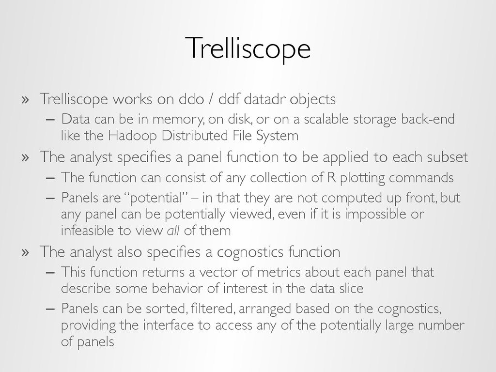
– Data can be in memory, on disk, or on a scalable storage back-end like the Hadoop Distributed File System » The analyst specifies a panel function to be applied to each subset – The function can consist of any collection of R plotting commands – Panels are “potential” – in that they are not computed up front, but any panel can be potentially viewed, even if it is impossible or infeasible to view all of them » The analyst also specifies a cognostics function – This function returns a vector of metrics about each panel that describe some behavior of interest in the data slice – Panels can be sorted, filtered, arranged based on the cognostics, providing the interface to access any of the potentially large number of panels
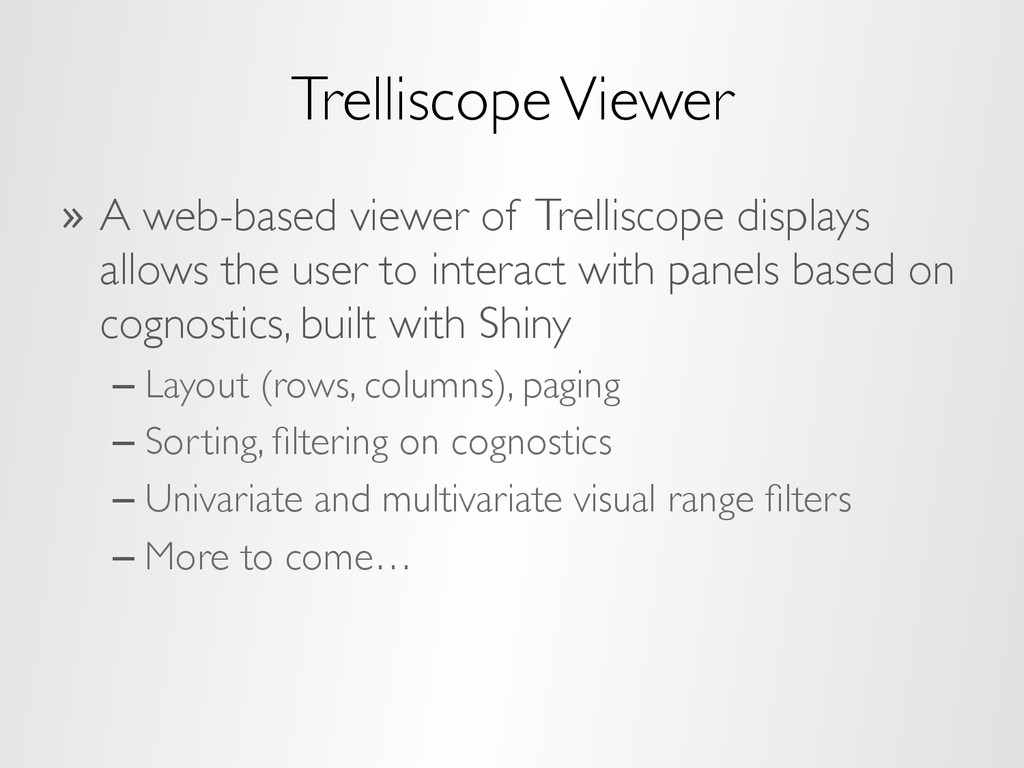
the user to interact with panels based on cognostics, built with Shiny – Layout (rows, columns), paging – Sorting, filtering on cognostics – Univariate and multivariate visual range filters – More to come…
votes agreeing w/ U.S. in each year (ignore abstain) – Plot them with a smooth local regression fit superposed » Ex: Afghanistan -->> 1990 1995 2000 2005 2010 0 20 40 60 80 100 Year Percentage of votes agreeing with U.S.
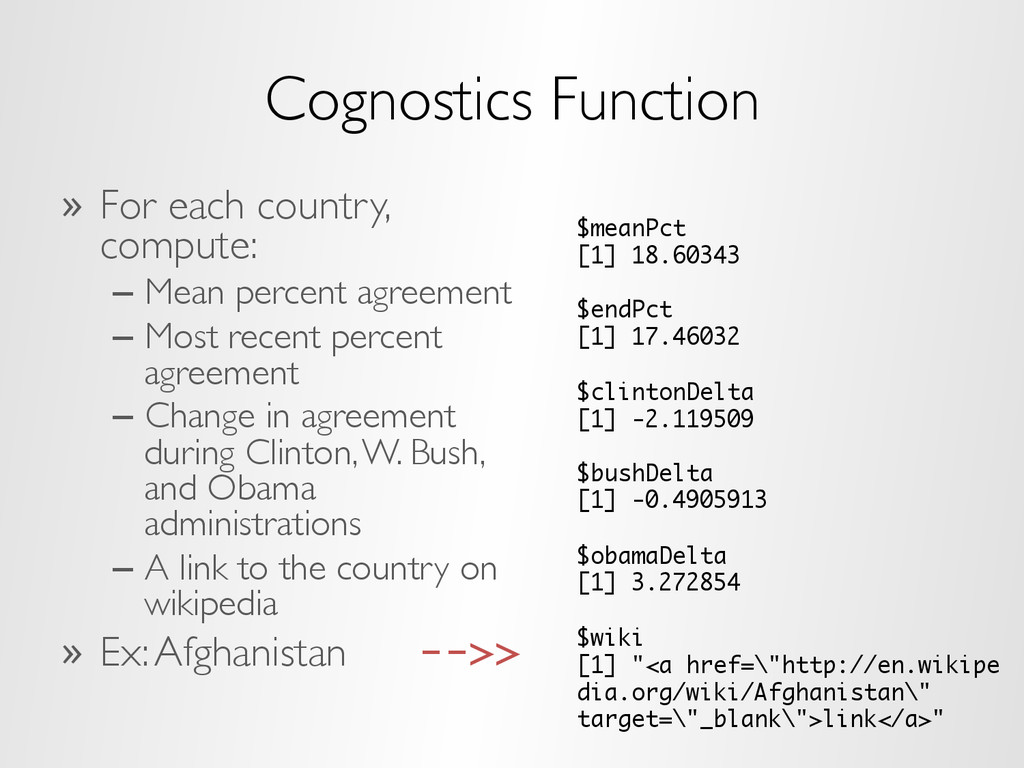
agreement – Most recent percent agreement – Change in agreement during Clinton, W. Bush, and Obama administrations – A link to the country on wikipedia » Ex: Afghanistan -->> $meanPct [1] 18.60343 $endPct [1] 17.46032 $clintonDelta [1] -2.119509 $bushDelta [1] -0.4905913 $obamaDelta [1] 3.272854 $wiki [1] "<a href=\"http://en.wikipe dia.org/wiki/Afghanistan\" target=\"_blank\">link</a>"
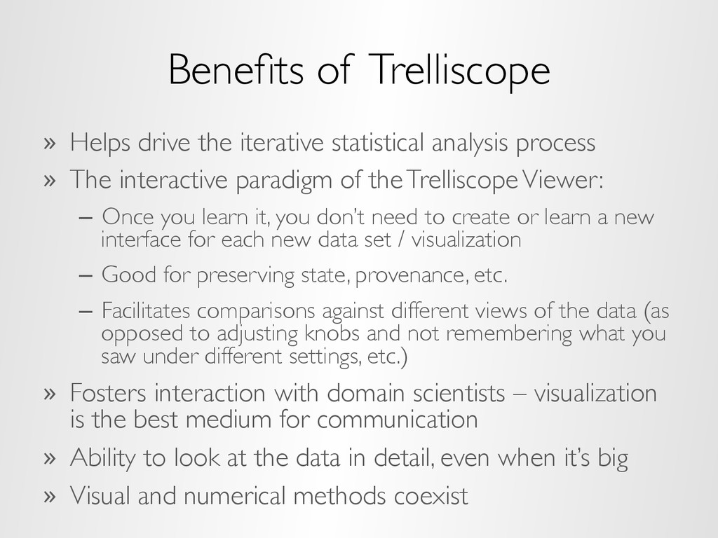
process » The interactive paradigm of the Trelliscope Viewer: – Once you learn it, you don’t need to create or learn a new interface for each new data set / visualization – Good for preserving state, provenance, etc. – Facilitates comparisons against different views of the data (as opposed to adjusting knobs and not remembering what you saw under different settings, etc.) » Fosters interaction with domain scientists – visualization is the best medium for communication » Ability to look at the data in detail, even when it’s big » Visual and numerical methods coexist
Apache license » Google user group » Start using it! – If you have some applications in mind, give it a try! – You don’t need big data or a cluster to use Tessera – Ask us for help, let us help you showcase your work – Give us feedback » See resources page in tessera.io » Theoretical / methodological research – There’s plenty of fertile ground
XDATA program » U.S. Department of Homeland Security, Science and Technology Directorate » Division of Math Sciences CDS&E Grant, National Science Foundation » PNNL, operated by Battelle for the U.S. Department of Energy, LDRD Program, Signature Discovery and Future Power Grid Initiatives
![“If [you have no] concern about error bars, about heterogeneity,](https://files.speakerdeck.com/presentations/7a968b904e9301329d885e31c290001e/slide_7.jpg)