-Heat-Exchanger-Design-SHELL AND TUBE

Transcript

1. Heat Exchanger Design Anand V P Gurumoorthy Associate Professor Chemical Engineering Division School of Mechanical & Building Sciences VIT University [EDITED BY AFRAZ ] ICET PU[UNIVERSITY OF THE PUNJAB LAHORE]
2. Heat Exchanger Classification •Recuperative: –Cold and hot fluid flow through the unit without mixing with each other. The transfer of heat occurs through the metal wall. •Regenerative: –Same heating surface is alternately exposed to hot and cold fluid. Heat from hot fluid is stored by packings or solids; this heat is passed over to the cold fluid. •Direct contact: –Hot and cold fluids are in direct contact and mixing occurs among them; mass transfer and heat transfer occur simultaneously.
3. Heat Exchanger Standards and Codes •British Standard BS-3274 •TEMA standards are universally used. •TEMA standards cover following classes of exchangers: –Class R – designates severe requirements of petroleum and other related processing applications –Class C – moderate requirements of commercial and general process applications –Class B – specifies design and fabrication for chemical process service.
4. Shell and Tube Heat Exchanger •Most commonly used type of heat transfer equipment in the chemical and allied industries. •Advantages: –The configuration gives a large surface area in a small volume. –Good mechanical layout: a good shape for pressure operation. –Uses well-established fabrication techniques. –Can be constructed from a wide range of materials. –Easily cleaned. –Well established design procedures.
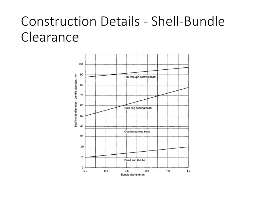
6. Types of Shell and Tube Heat Exchangers •Fixed tube design –Simplest and cheapest type. –Tube bundle cannot be removed for cleaning. –No provision for differential expansion of shell and tubes. –Use of this type limited to temperature difference upto 800C. •Floating head design –More versatile than fixed head exchangers. –Suitable for higher temperature differentials. –Bundles can be removed and cleaned (fouling liquids)
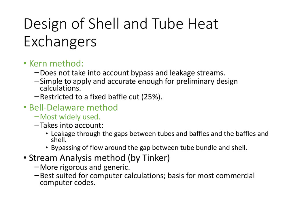
7. Design of Shell and Tube Heat Exchangers • Kern method: –Does not take into account bypass and leakage streams. –Simple to apply and accurate enough for preliminary design calculations. –Restricted to a fixed baffle cut (25%). • Bell-Delaware method –Most widely used. –Takes into account: • Leakage through the gaps between tubes and baffles and the baffles and shell. • Bypassing of flow around the gap between tube bundle and shell. • Stream Analysis method (by Tinker) –More rigorous and generic. –Best suited for computer calculations; basis for most commercial computer codes.
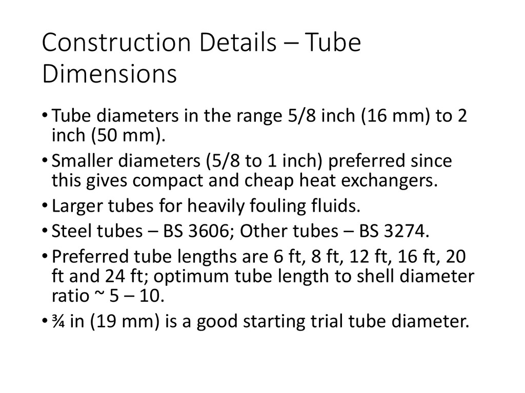
8. Construction Details – Tube Dimensions •Tube diameters in the range 5/8 inch (16 mm) to 2 inch (50 mm). •Smaller diameters (5/8 to 1 inch) preferred since this gives compact and cheap heat exchangers. •Larger tubes for heavily fouling fluids. •Steel tubes – BS 3606; Other tubes – BS 3274. •Preferred tube lengths are 6 ft, 8 ft, 12 ft, 16 ft, 20 ft and 24 ft; optimum tube length to shell diameter ratio ~ 5 – 10. •¾ in (19 mm) is a good starting trial tube diameter.
9. Construction Details – Tube Arrangements • Tubes usually arranged in equilateral triangular, square or rotated square patterns. • Tube pitch, Pt , is 1.25 times OD.
10. Construction Details - Shells • Shell should be a close fit to the tube bundle to reduce bypassing. • Shell-bundle clearance will depend on type of heat exchanger.
11. Construction Details - Shell-Bundle Clearance
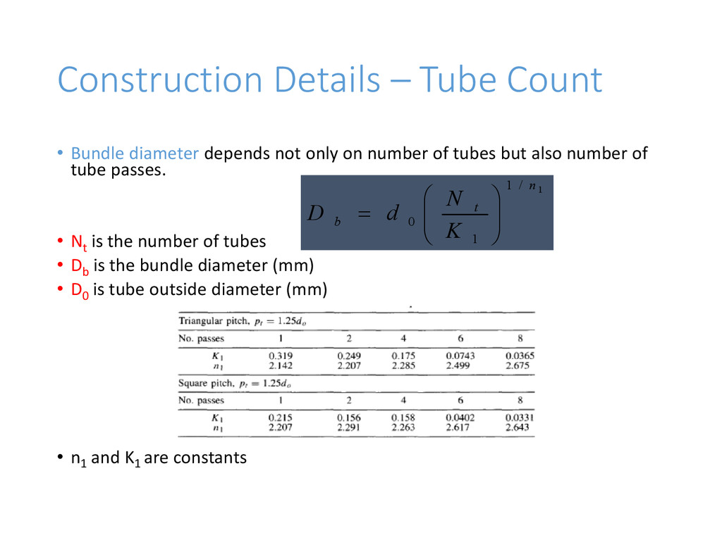
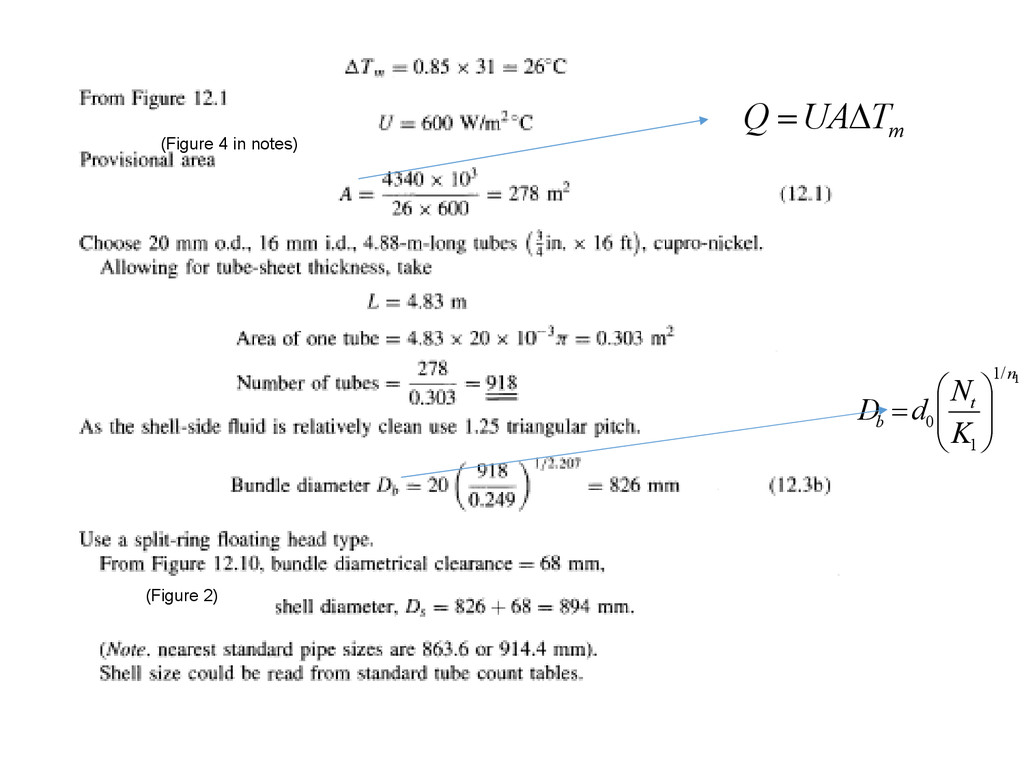
12. Construction Details – Tube Count • Bundle diameter depends not only on number of tubes but also number of tube passes. • Nt is the number of tubes • Db is the bundle diameter (mm) • D0 is tube outside diameter (mm) • n1 and K1 are constants 1 / 1 1 0 n t b K N d D         
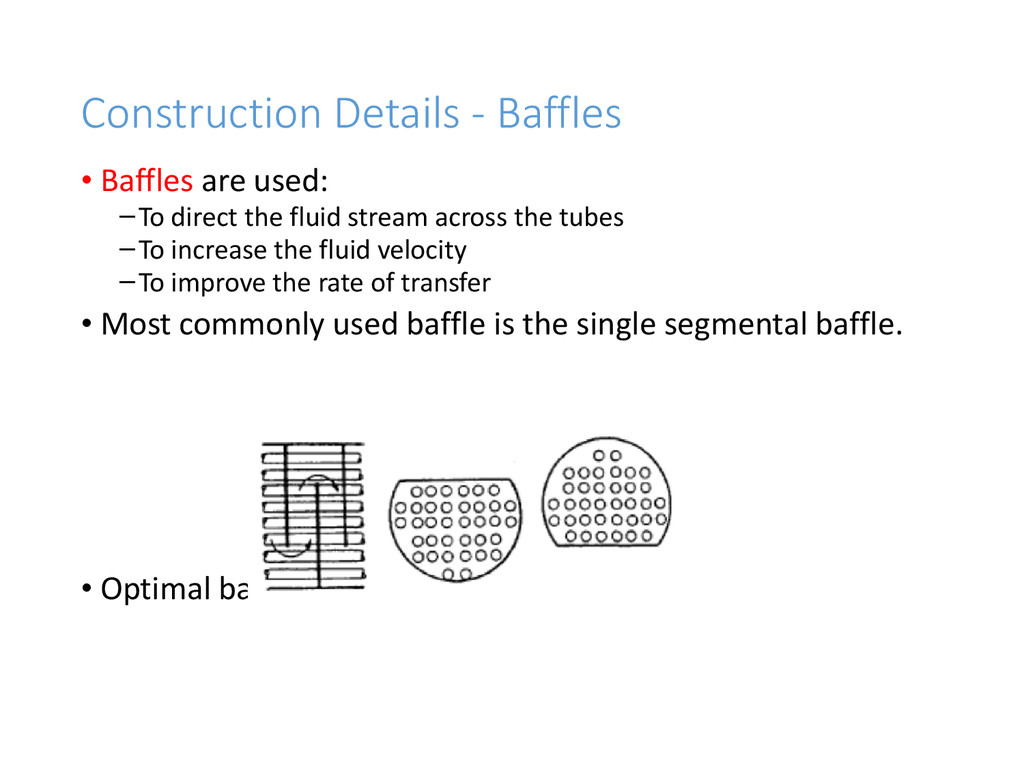
13. Construction Details - Baffles • Baffles are used: –To direct the fluid stream across the tubes –To increase the fluid velocity –To improve the rate of transfer • Most commonly used baffle is the single segmental baffle. • Optimal baffle cut ~ 20-25%
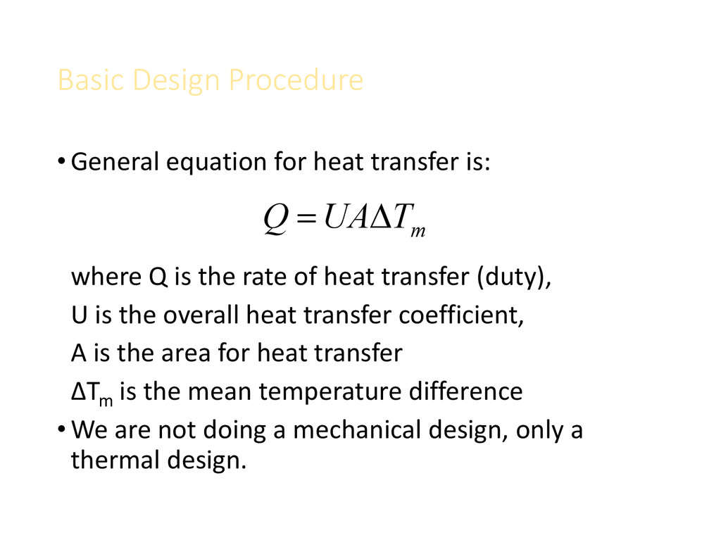
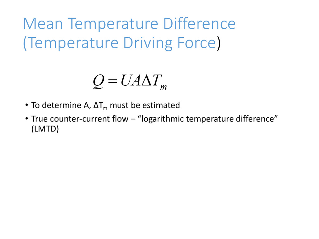
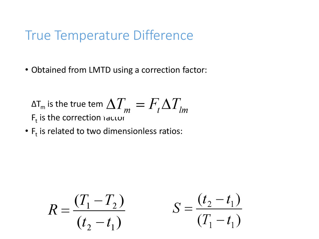
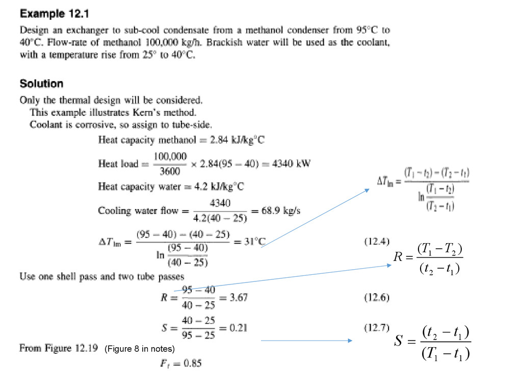
14. Basic Design Procedure •General equation for heat transfer is: where Q is the rate of heat transfer (duty), U is the overall heat transfer coefficient, A is the area for heat transfer ΔTm is the mean temperature difference •We are not doing a mechanical design, only a thermal design. m T UA Q  
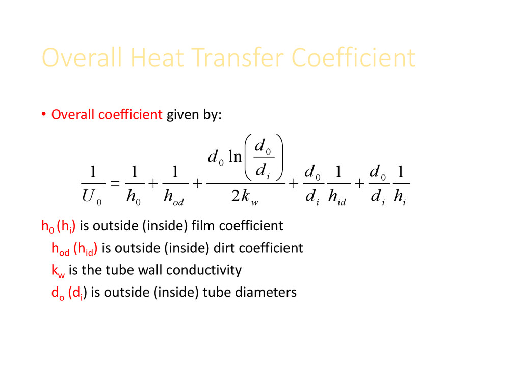
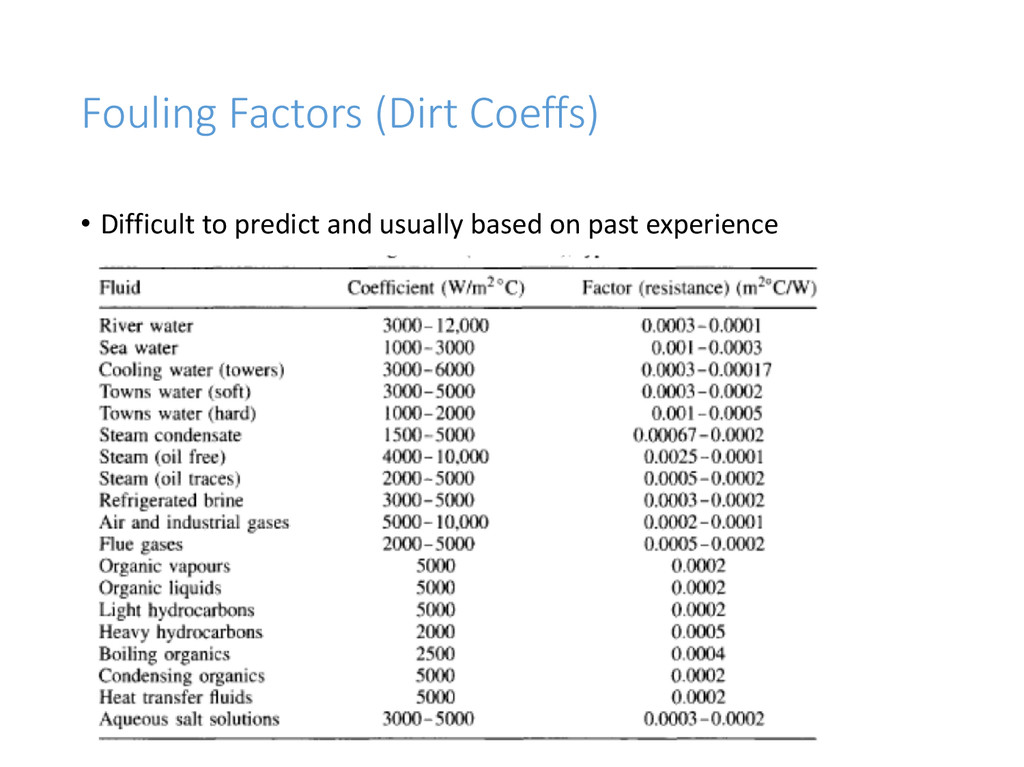
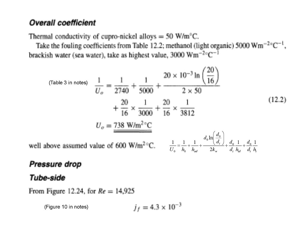
15. Overall Heat Transfer Coefficient • Overall coefficient given by: h0 (hi ) is outside (inside) film coefficient hod (hid ) is outside (inside) dirt coefficient kw is the tube wall conductivity do (di ) is outside (inside) tube diameters i i id i w i od h d d h d d k d d d h h U 1 1 2 ln 1 1 1 0 0 0 0 0 0             
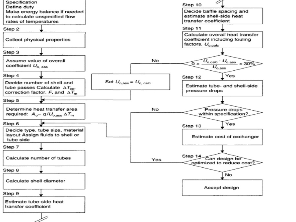
16. Individual Film Coefficients •Magnitude of individual coefficients will depend on: –Nature of transfer processes (conduction, convection, radiation, etc.) –Physical properties of fluids –Fluid flow rates –Physical layout of heat transfer surface •Physical layout cannot be determined until area is known; hence design is a trial-and-error procedure.
17. Typical Overall Coefficients
18. Typical Overall Coefficients
19. Fouling Factors (Dirt Coeffs) • Difficult to predict and usually based on past experience
20. Mean Temperature Difference (Temperature Driving Force) • To determine A, ΔTm must be estimated • True counter-current flow – “logarithmic temperature difference” (LMTD) m T UA Q  
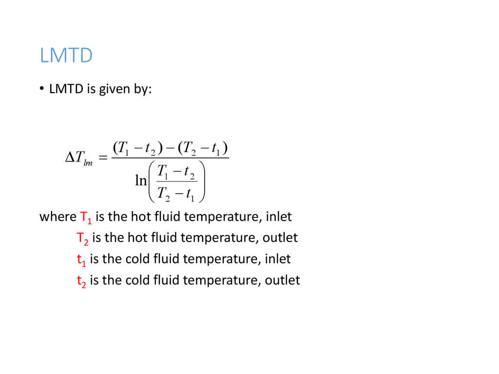
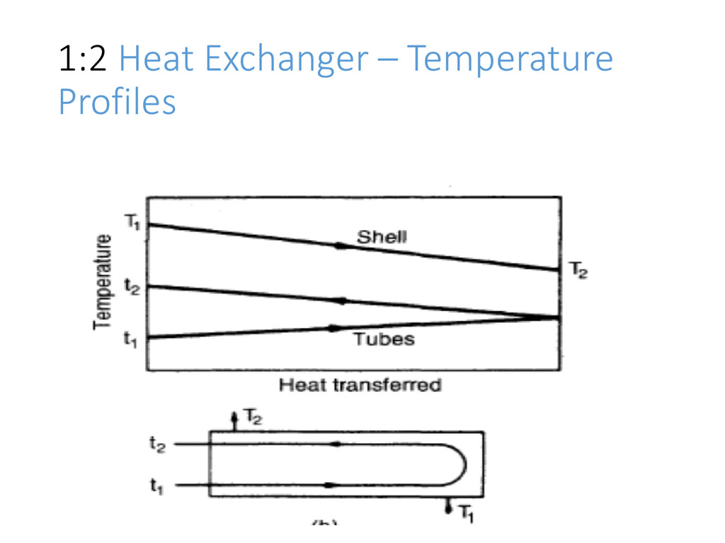
21. LMTD • LMTD is given by: where T1 is the hot fluid temperature, inlet T2 is the hot fluid temperature, outlet t1 is the cold fluid temperature, inlet t2 is the cold fluid temperature, outlet                1 2 2 1 1 2 2 1 ln ) ( ) ( t T t T t T t T Tlm
22. Counter-current Flow – Temperature Proflies
23. 1:2 Heat Exchanger – Temperature Profiles
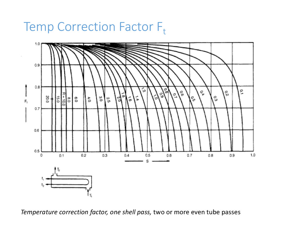
24. True Temperature Difference • Obtained from LMTD using a correction factor: ΔTm is the true temperature difference Ft is the correction factor • Ft is related to two dimensionless ratios: lm t m T F T    ) ( ) ( 1 2 2 1 t t T T R    ) ( ) ( 1 1 1 2 t T t t S   
25. Temp Correction Factor Ft Temperature correction factor, one shell pass, two or more even tube passes
26. Fluid Allocation: Shell or Tubes? • Corrosion • Fouling • Fluid temperatures • Operating pressures • Pressure drop • Viscosity • Stream flow rates
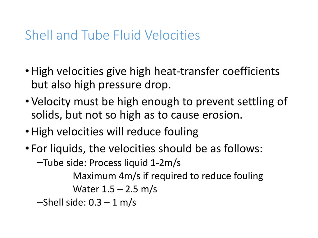
27. Shell and Tube Fluid Velocities •High velocities give high heat-transfer coefficients but also high pressure drop. •Velocity must be high enough to prevent settling of solids, but not so high as to cause erosion. •High velocities will reduce fouling •For liquids, the velocities should be as follows: –Tube side: Process liquid 1-2m/s Maximum 4m/s if required to reduce fouling Water 1.5 – 2.5 m/s –Shell side: 0.3 – 1 m/s
28. Pressure Drop • As the process fluids move through the heat exchanger there is associated pressure drop. • For liquids: viscosity < 1mNs/m2 35kN/m2 Viscosity 1 – 10 mNs/m2 50-70kN/m2
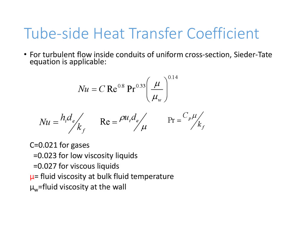
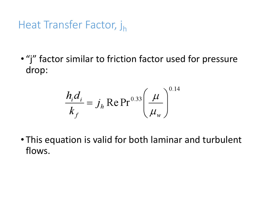
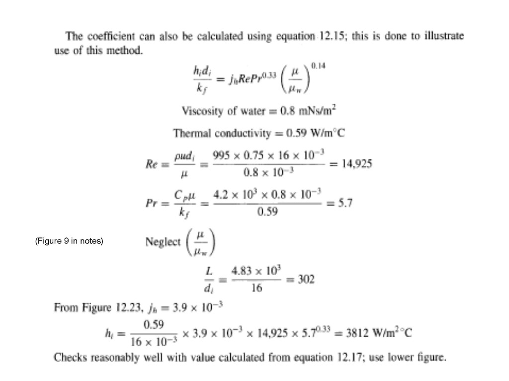
29. Tube-side Heat Transfer Coefficient • For turbulent flow inside conduits of uniform cross-section, Sieder-Tate equation is applicable: C=0.021 for gases =0.023 for low viscosity liquids =0.027 for viscous liquids μ= fluid viscosity at bulk fluid temperature μw =fluid viscosity at the wall 14 . 0 33 . 0 8 . 0 Pr Re          w C Nu   f e i k d h Nu    e t d u  Re f p k C   Pr
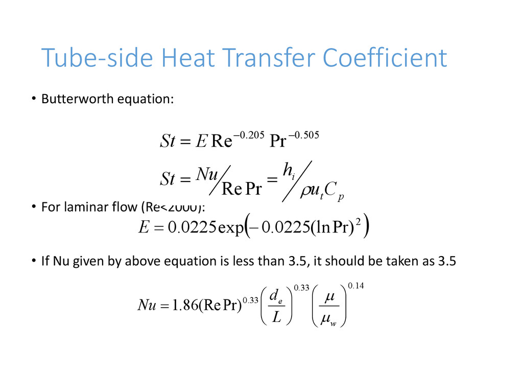
30. Tube-side Heat Transfer Coefficient • Butterworth equation: • For laminar flow (Re<2000): • If Nu given by above equation is less than 3.5, it should be taken as 3.5 505 . 0 205 . 0 Pr Re    E St p t i C u h Nu St    Pr Re   2 Pr) (ln 0225 . 0 exp 0225 . 0   E 14 . 0 33 . 0 33 . 0 Pr) (Re 86 . 1                w e L d Nu  
31. Heat Transfer Factor, jh •“j” factor similar to friction factor used for pressure drop: •This equation is valid for both laminar and turbulent flows. 14 . 0 33 . 0 Pr Re          w h f i i j k d h  
32. Tube Side Heat Transfer Factor
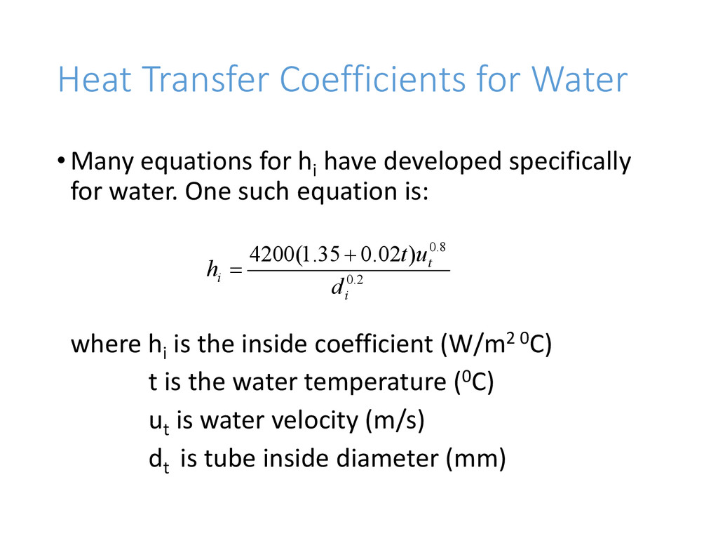
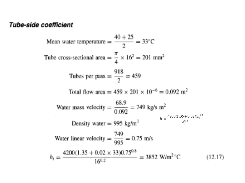
33. Heat Transfer Coefficients for Water •Many equations for hi have developed specifically for water. One such equation is: where hi is the inside coefficient (W/m2 0C) t is the water temperature (0C) ut is water velocity (m/s) dt is tube inside diameter (mm) 2 . 0 8 . 0 ) 02 . 0 35 . 1 ( 4200 i t i d u t h  
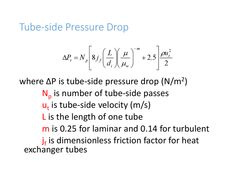
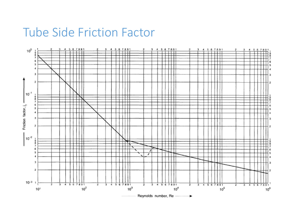
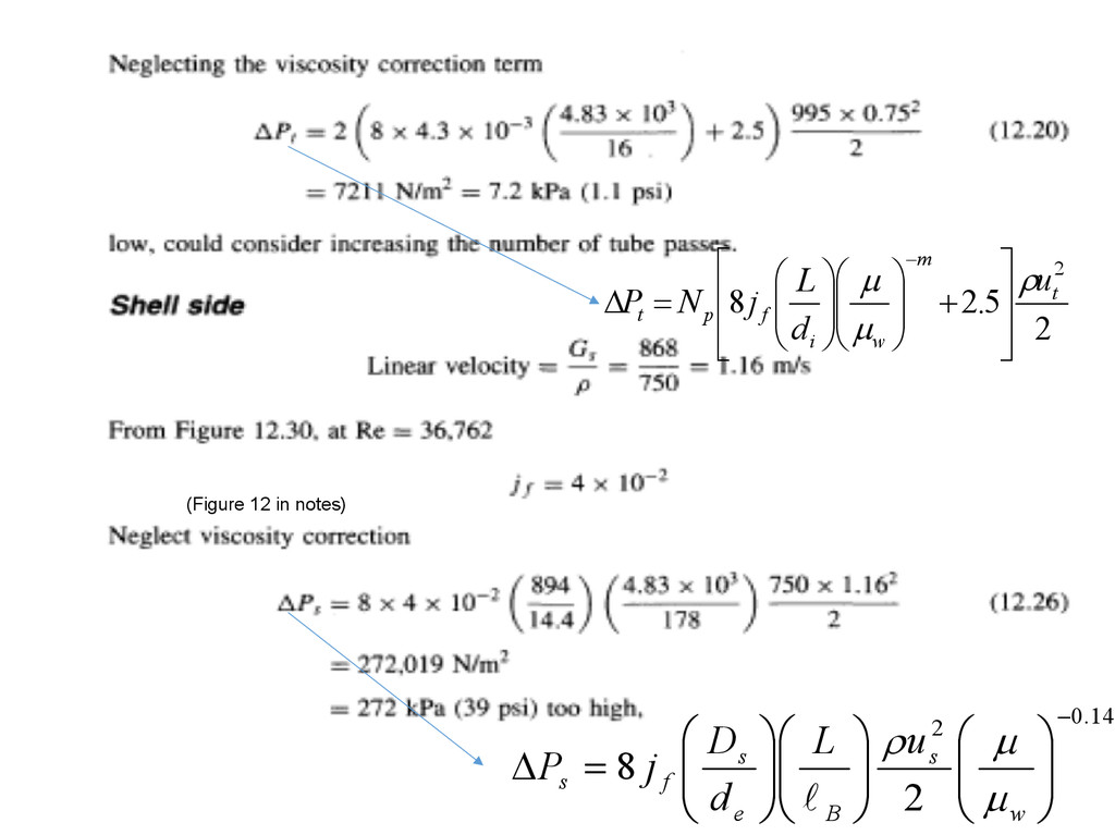
34. Tube-side Pressure Drop where ΔP is tube-side pressure drop (N/m2) Np is number of tube-side passes ut is tube-side velocity (m/s) L is the length of one tube m is 0.25 for laminar and 0.14 for turbulent jf is dimensionless friction factor for heat exchanger tubes 2 5 . 2 8 2 t m w i f p t u d L j N P                               
35. Tube Side Friction Factor
36. Shell-side Heat Transfer and Pressure Drop •Kern’s method •Bell’s method
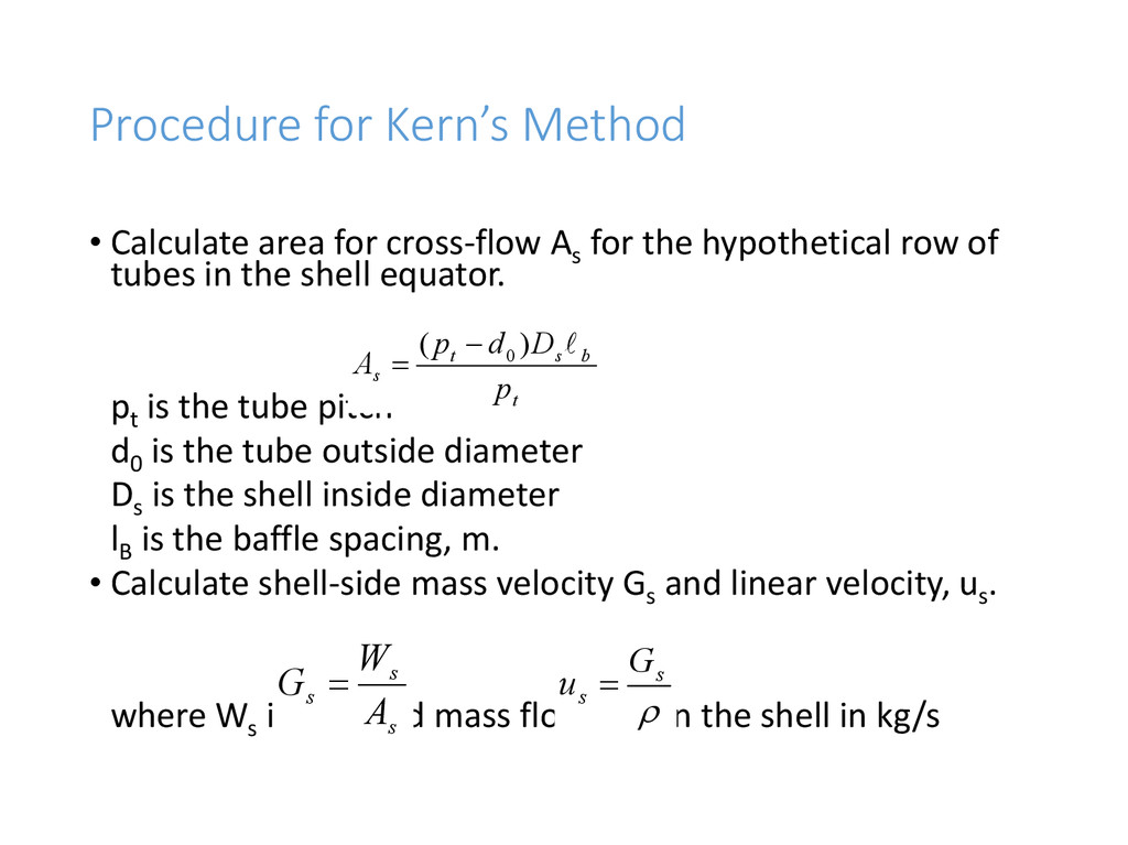
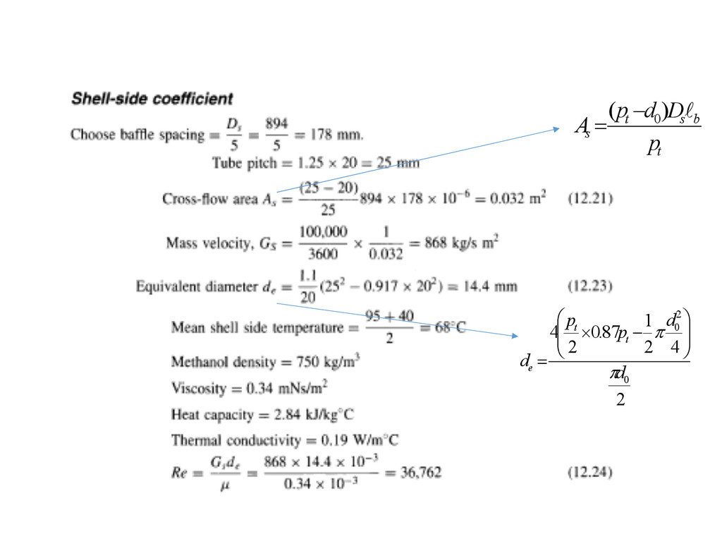
38. Procedure for Kern’s Method • Calculate area for cross-flow As for the hypothetical row of tubes in the shell equator. pt is the tube pitch d0 is the tube outside diameter Ds is the shell inside diameter lB is the baffle spacing, m. • Calculate shell-side mass velocity Gs and linear velocity, us . where Ws is the fluid mass flow rate in the shell in kg/s t b s t s p D d p A  ) ( 0   s s s A W G   s s G u 
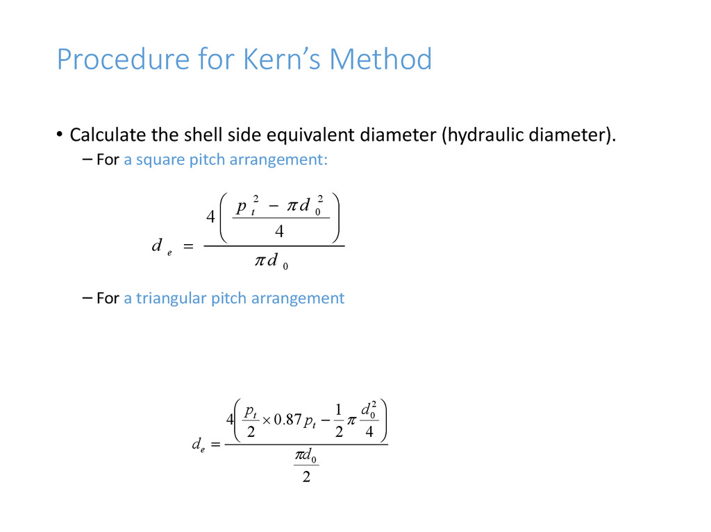
39. Procedure for Kern’s Method • Calculate the shell side equivalent diameter (hydraulic diameter). – For a square pitch arrangement: – For a triangular pitch arrangement 0 2 0 2 4 4 d d p d t e             2 4 2 1 87 . 0 2 4 0 2 0 d d p p d t t e             
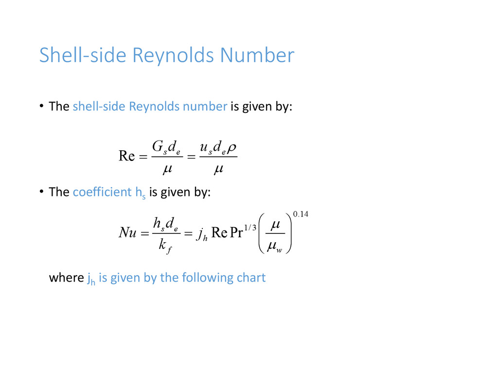
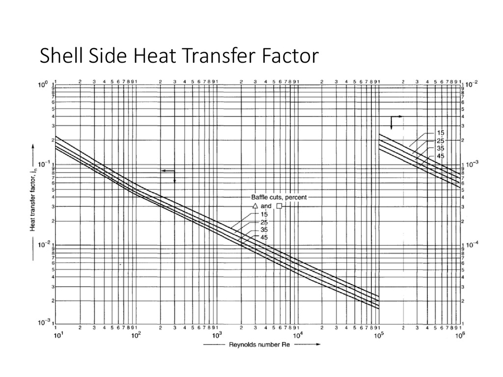
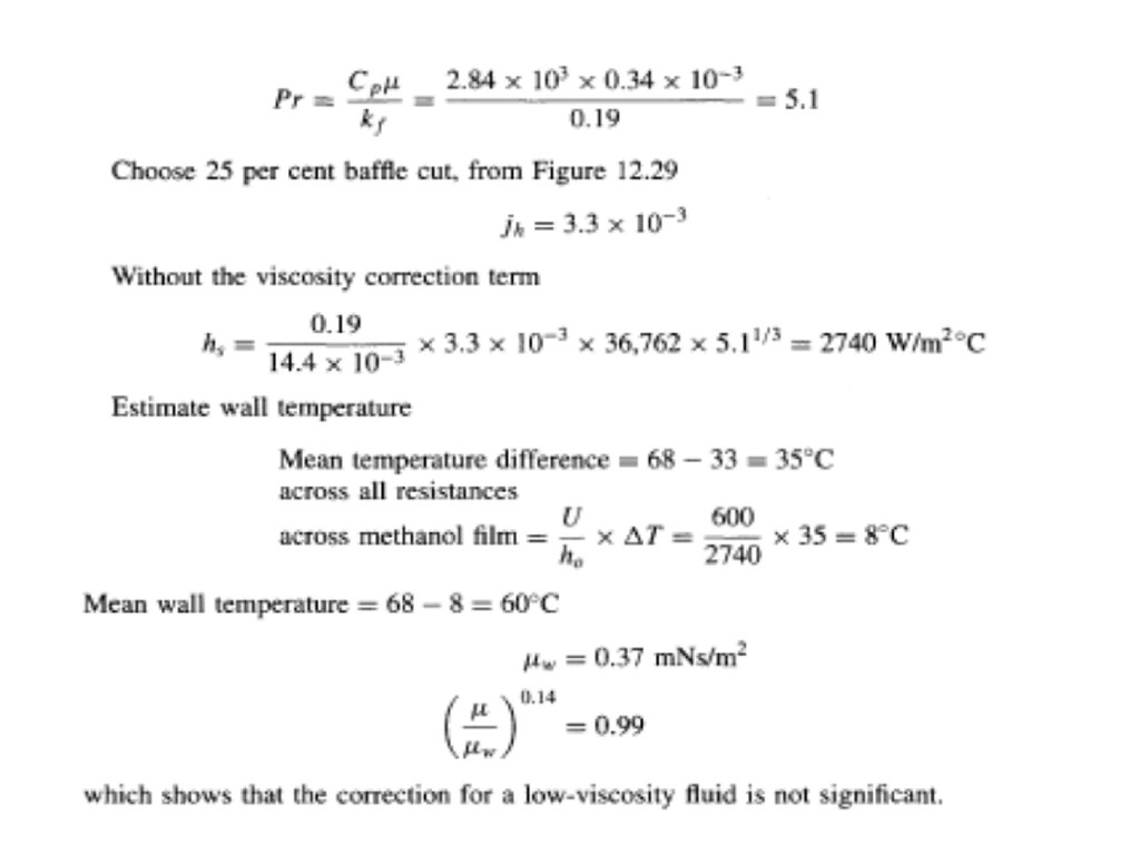
40. Shell-side Reynolds Number • The shell-side Reynolds number is given by: • The coefficient hs is given by: where jh is given by the following chart    e s e s d u d G   Re 14 . 0 3 / 1 Pr Re           w h f e s j k d h Nu  
41. Shell Side Heat Transfer Factor
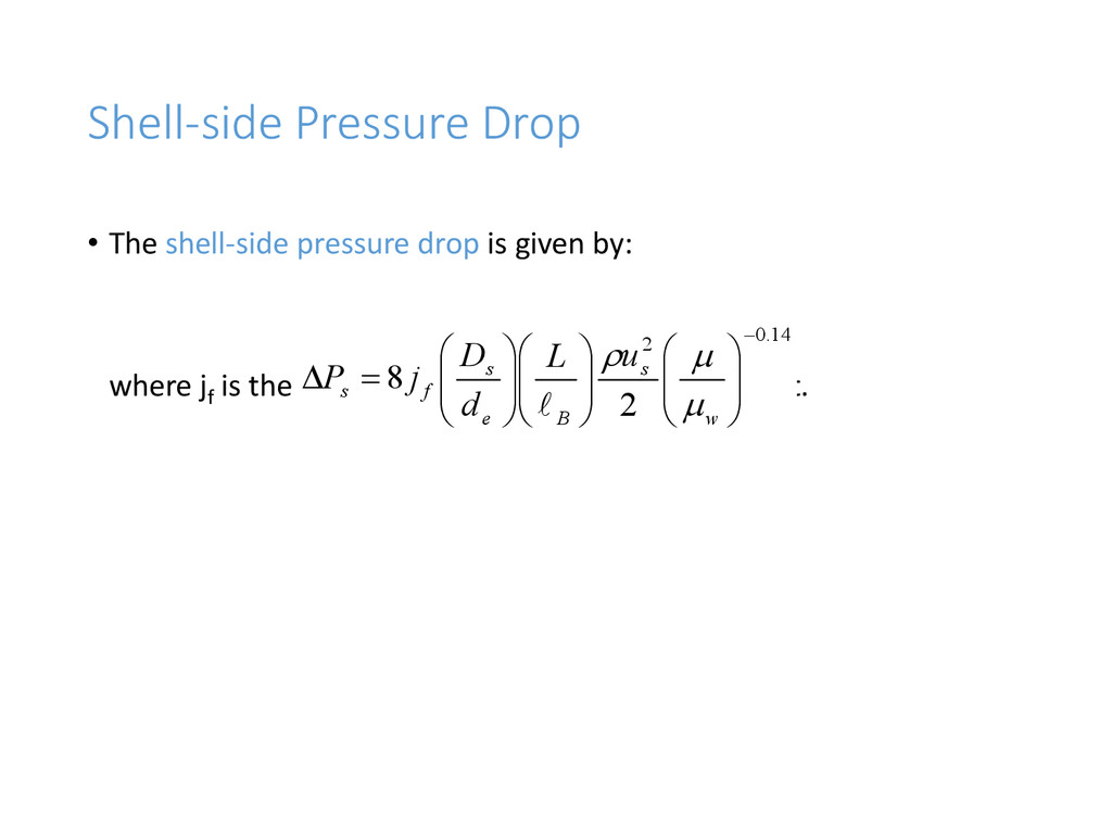
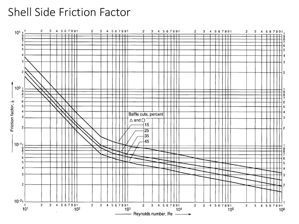
42. Shell-side Pressure Drop • The shell-side pressure drop is given by: where jf is the friction factor given by following chart. 14 . 0 2 2 8                            w s B e s f s u L d D j P    
43. Shell Side Friction Factor
44. ) ( ) ( 1 2 2 1 t t T T R    ) ( ) ( 1 1 1 2 t T t t S    (Figure 8 in notes)
45. m T UA Q   1 / 1 1 0 n t b K N d D          (Figure 4 in notes) (Figure 2)
46. 2 . 0 8 . 0 ) 02 . 0 35 . 1 ( 4200 i t i d u t h  
47. (Figure 9 in notes)
48. t b s t s p D d p A  ) ( 0   2 4 2 1 87 . 0 2 4 0 2 0 d d p p d t t e             
50. i i id i w i od h d d h d d k d d d h h U 1 1 2 ln 1 1 1 0 0 0 0 0 0              (Figure 10 in notes) (Table 3 in notes)
51. 2 5 . 2 8 2 t m w i f p t u d L j N P                                14 . 0 2 2 8                            w s B e s f s u L d D j P     (Figure 12 in notes)
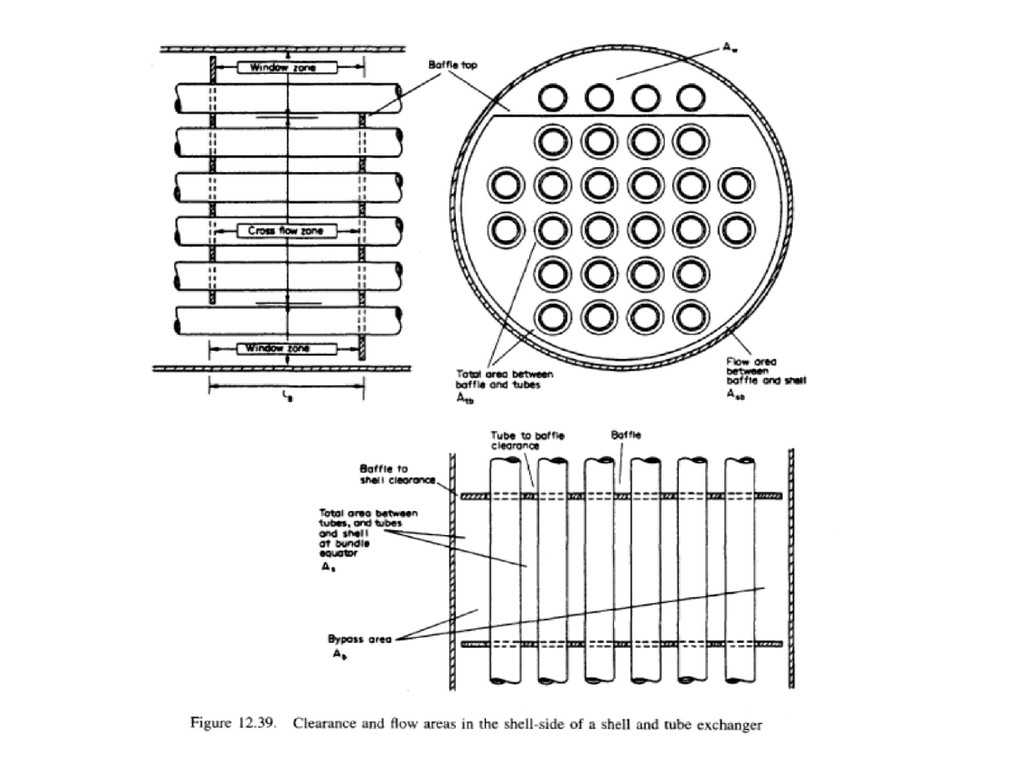
53. Bell’s Method • In Bell’s method, the heat transfer coefficient and pressure drop are estimated from correlations for flow over ideal tube banks. • The effects of leakage, by-passing, and flow in the window zone are allowed for by applying correction factors.
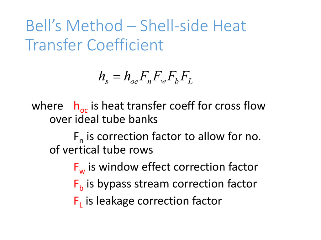
54. Bell’s Method – Shell-side Heat Transfer Coefficient where hoc is heat transfer coeff for cross flow over ideal tube banks Fn is correction factor to allow for no. of vertical tube rows Fw is window effect correction factor Fb is bypass stream correction factor FL is leakage correction factor L b w n oc s F F F F h h 
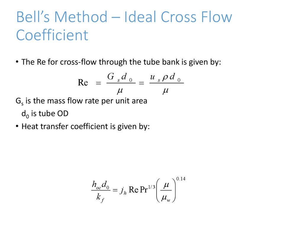
57. Bell’s Method – Ideal Cross Flow Coefficient • The Re for cross-flow through the tube bank is given by: Gs is the mass flow rate per unit area d0 is tube OD • Heat transfer coefficient is given by:    0 0 Re d u d G s s   14 . 0 3 / 1 0 Pr Re          w h f oc j k d h  
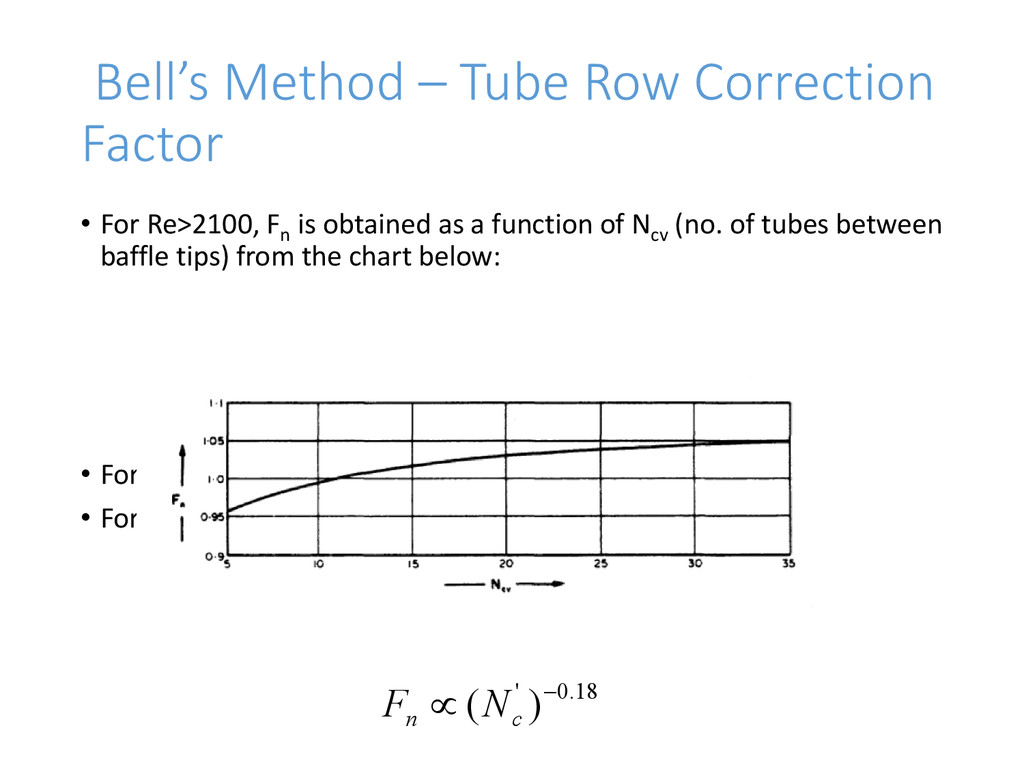
58. Bell’s Method – Tube Row Correction Factor • For Re>2100, Fn is obtained as a function of Ncv (no. of tubes between baffle tips) from the chart below: • For Re 100<Re<2100, Fn =1.0 • For Re<100, 18 . 0 ' ) (   c n N F
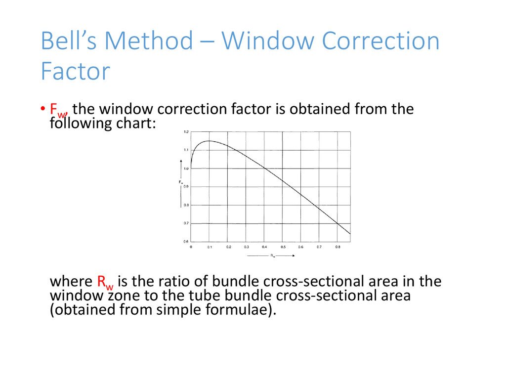
59. Bell’s Method – Window Correction Factor • Fw , the window correction factor is obtained from the following chart: where Rw is the ratio of bundle cross-sectional area in the window zone to the tube bundle cross-sectional area (obtained from simple formulae).
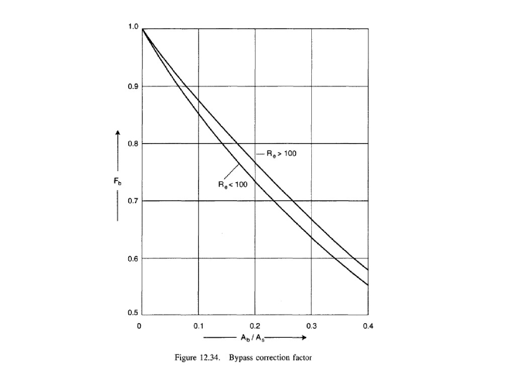
60. Bell’s Method – Bypass Correction Factor • Clearance area[Ab] between the bundle and the shell • For the case of no sealing strips, Fb as a function of Ab /As can be obtained from the following chart ) ( b s B b D D A   
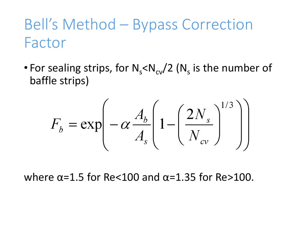
62. Bell’s Method – Bypass Correction Factor •For sealing strips, for Ns <Ncv /2 (Ns is the number of baffle strips) where α=1.5 for Re<100 and α=1.35 for Re>100.                            3 / 1 2 1 exp cv s s b b N N A A F 
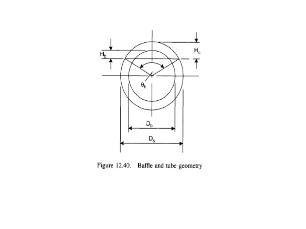
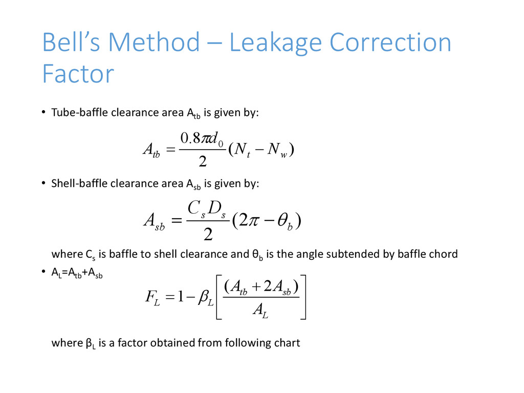
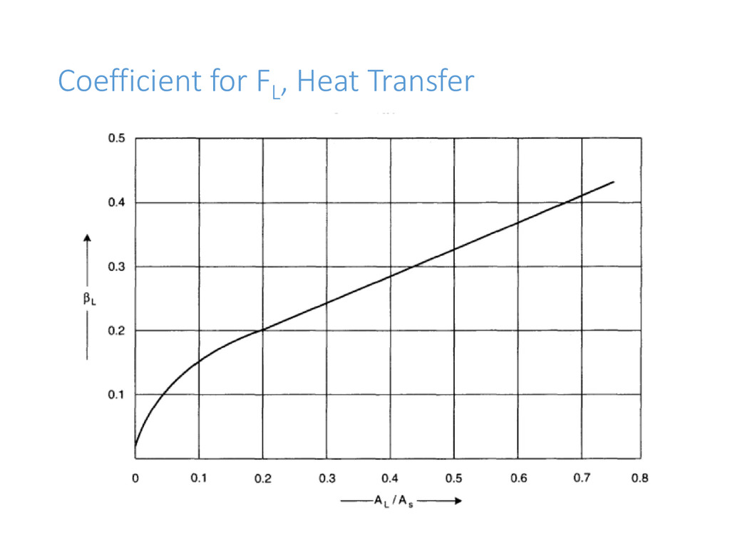
63. Bell’s Method – Leakage Correction Factor • Tube-baffle clearance area Atb is given by: • Shell-baffle clearance area Asb is given by: where Cs is baffle to shell clearance and θb is the angle subtended by baffle chord • AL =Atb +Asb where βL is a factor obtained from following chart ) ( 2 8 . 0 0 w t tb N N d A    ) 2 ( 2 b s s sb D C A              L sb tb L L A A A F ) 2 ( 1 
64. Coefficient for FL , Heat Transfer
65. Shell-side Pressure Drop • Involves three components: – Pressure drop in cross-flow zone – Pressure drop in window zone – Pressure drop in end zone
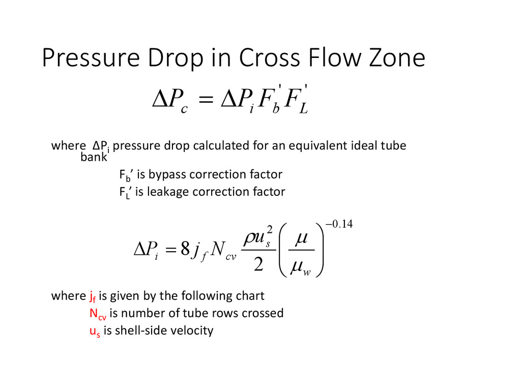
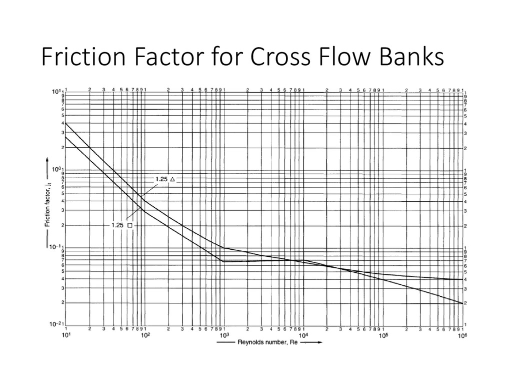
66. Pressure Drop in Cross Flow Zone where ΔPi pressure drop calculated for an equivalent ideal tube bank Fb ’ is bypass correction factor FL ’ is leakage correction factor where jf is given by the following chart Ncv is number of tube rows crossed us is shell-side velocity ' ' L b i c F F P P    14 . 0 2 2 8            w s cv f i u N j P   
67. Friction Factor for Cross Flow Banks
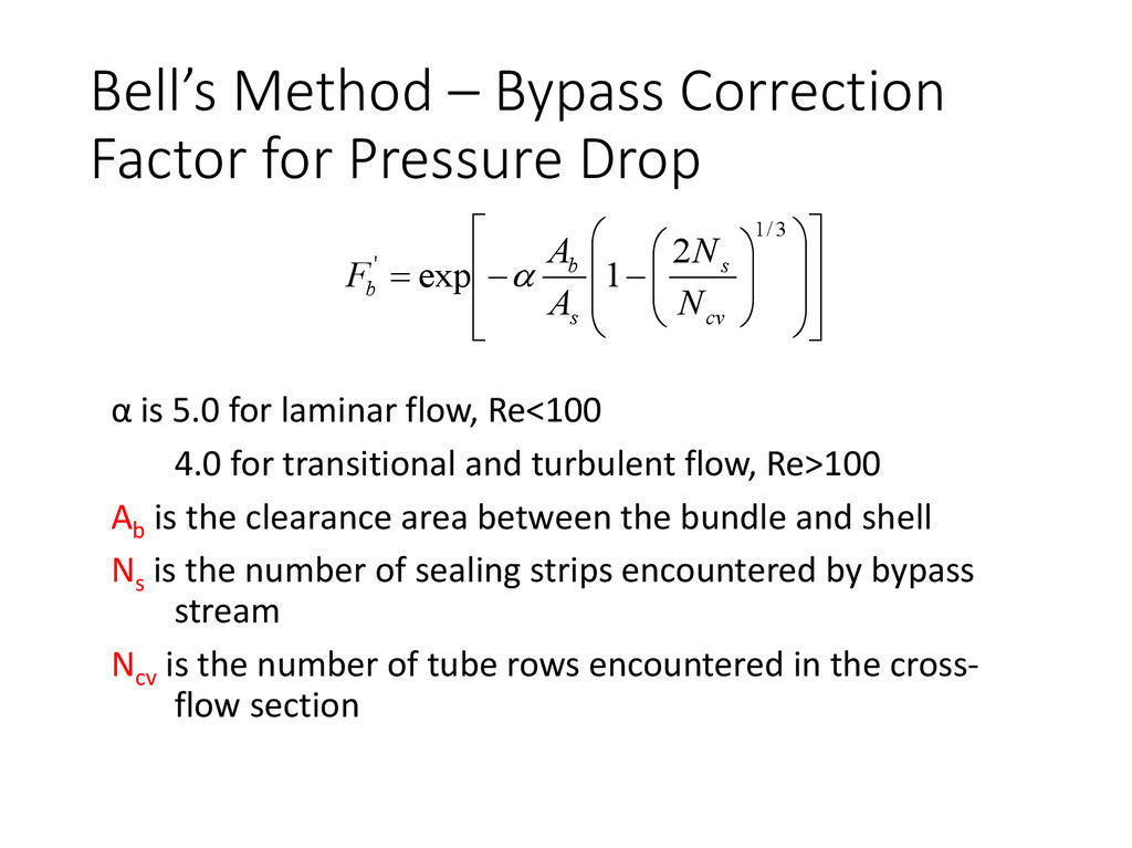
68. Bell’s Method – Bypass Correction Factor for Pressure Drop α is 5.0 for laminar flow, Re<100 4.0 for transitional and turbulent flow, Re>100 Ab is the clearance area between the bundle and shell Ns is the number of sealing strips encountered by bypass stream Ncv is the number of tube rows encountered in the cross- flow section                            3 / 1 ' 2 1 exp cv s s b b N N A A F 
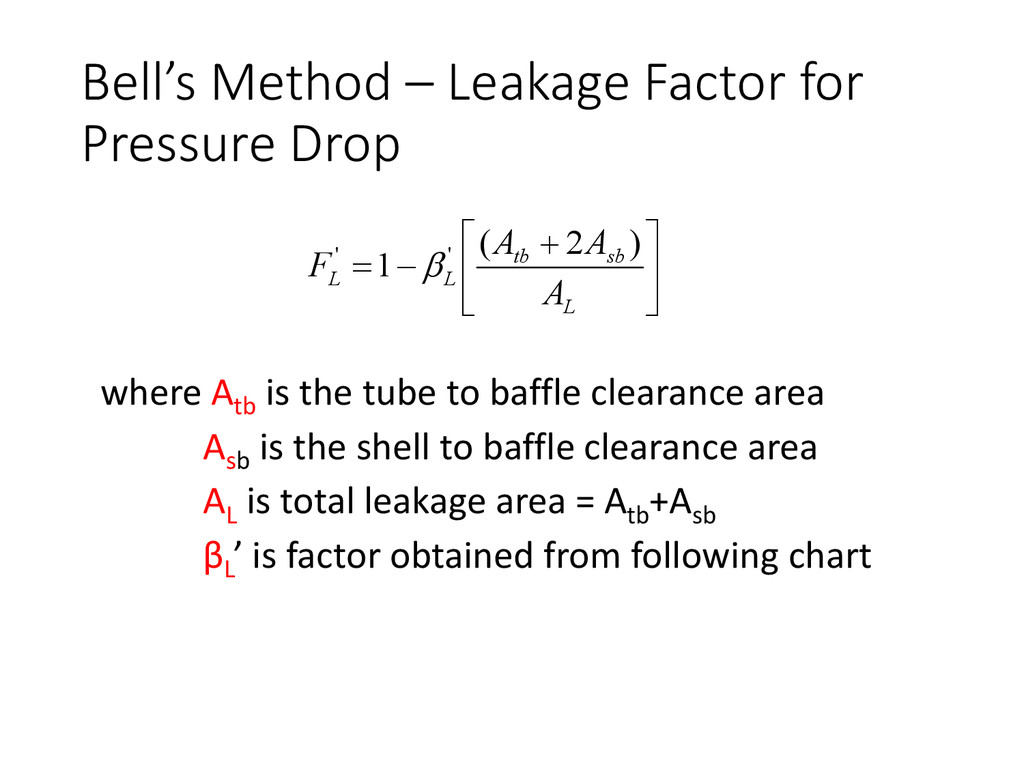
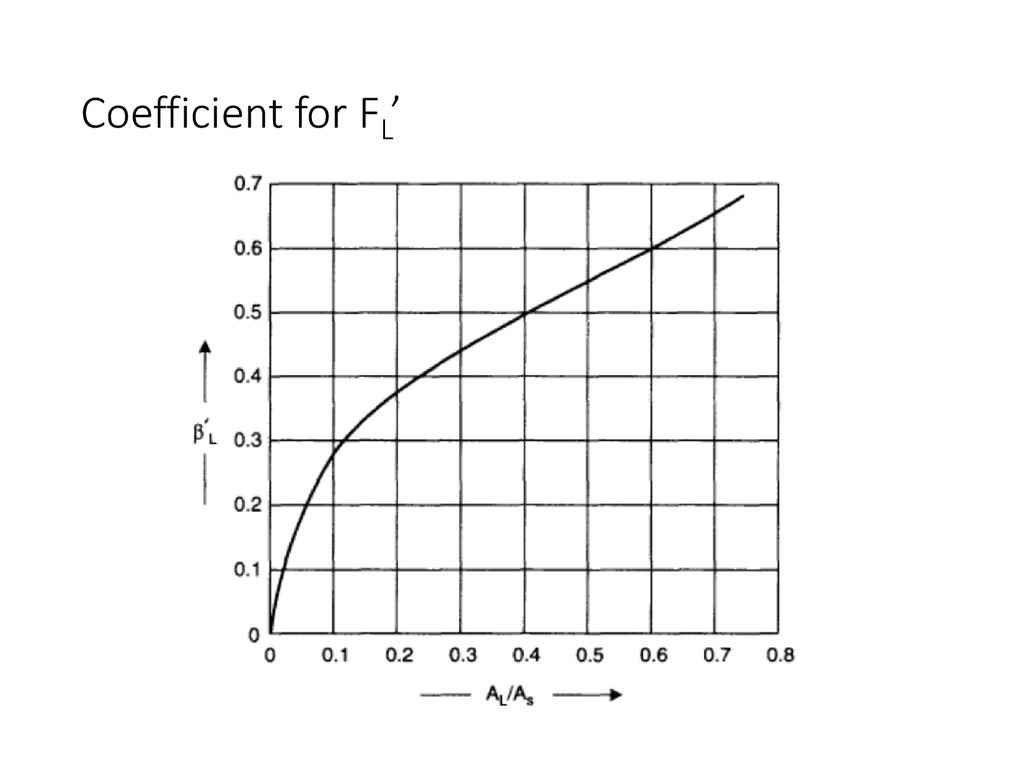
69. Bell’s Method – Leakage Factor for Pressure Drop where Atb is the tube to baffle clearance area Asb is the shell to baffle clearance area AL is total leakage area = Atb +Asb βL ’ is factor obtained from following chart          L sb tb L L A A A F ) 2 ( 1 ' ' 
70. Coefficient for FL ’
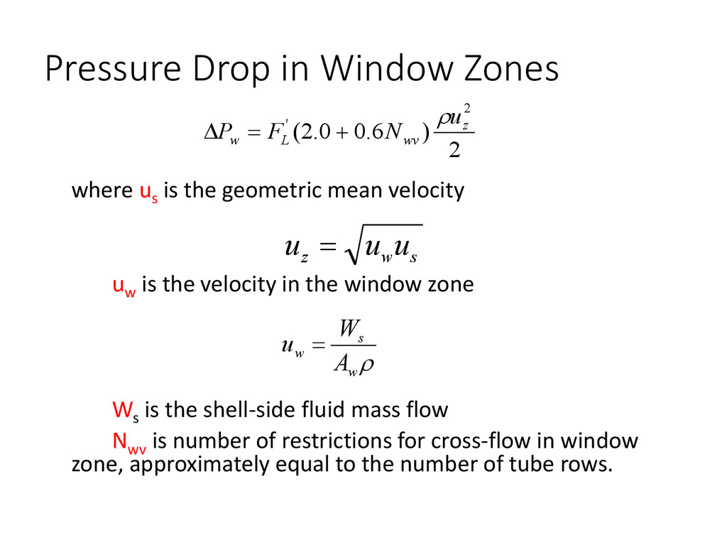
71. Pressure Drop in Window Zones where us is the geometric mean velocity uw is the velocity in the window zone Ws is the shell-side fluid mass flow Nwv is number of restrictions for cross-flow in window zone, approximately equal to the number of tube rows. 2 ) 6 . 0 0 . 2 ( 2 ' z wv L w u N F P     s w z u u u   w s w A W u 
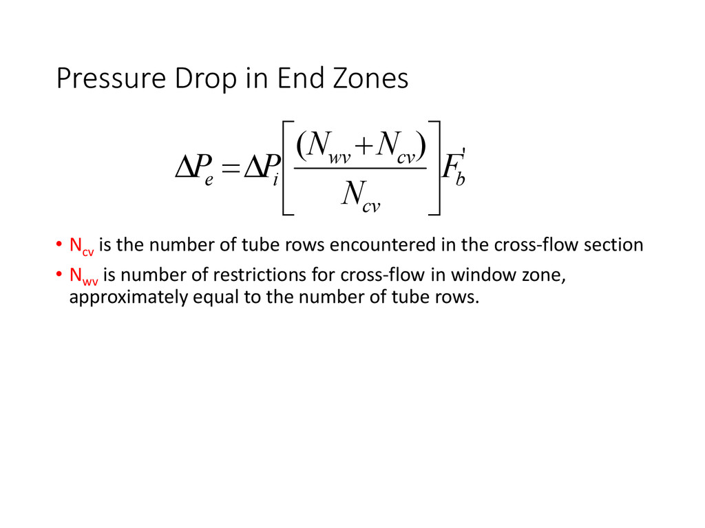
72. Pressure Drop in End Zones • Ncv is the number of tube rows encountered in the cross-flow section • Nwv is number of restrictions for cross-flow in window zone, approximately equal to the number of tube rows. ' ) ( b cv cv wv i e F N N N P P          
73. Bell’s Method – Total Shell-side Pressure Drop zones window N zones crossflow N zones end P b b s      ) 1 ( 2 w b c b e s P N P N P P         ) 1 ( 2
74. Effect of Fouling • Above calculation assumes clean tubes • Effect of fouling on pressure drop is given by table above
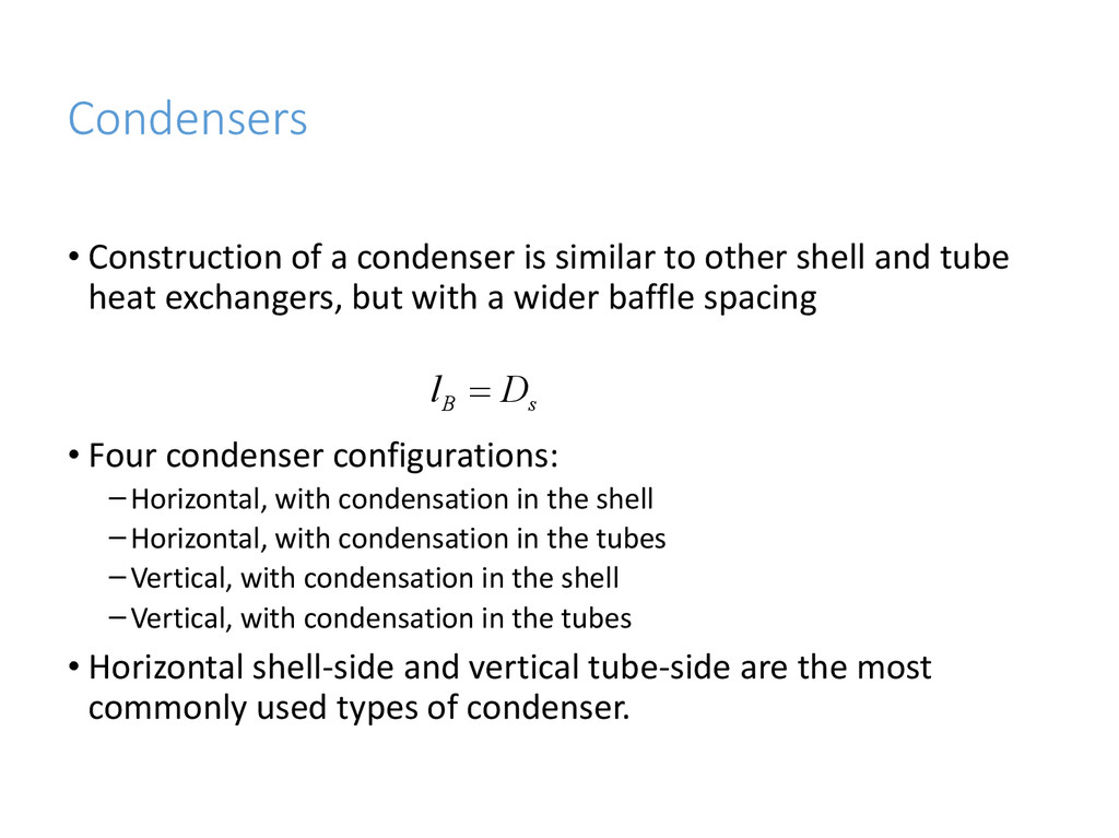
75. Condensers • Construction of a condenser is similar to other shell and tube heat exchangers, but with a wider baffle spacing • Four condenser configurations: –Horizontal, with condensation in the shell –Horizontal, with condensation in the tubes –Vertical, with condensation in the shell –Vertical, with condensation in the tubes • Horizontal shell-side and vertical tube-side are the most commonly used types of condenser. s B D l 
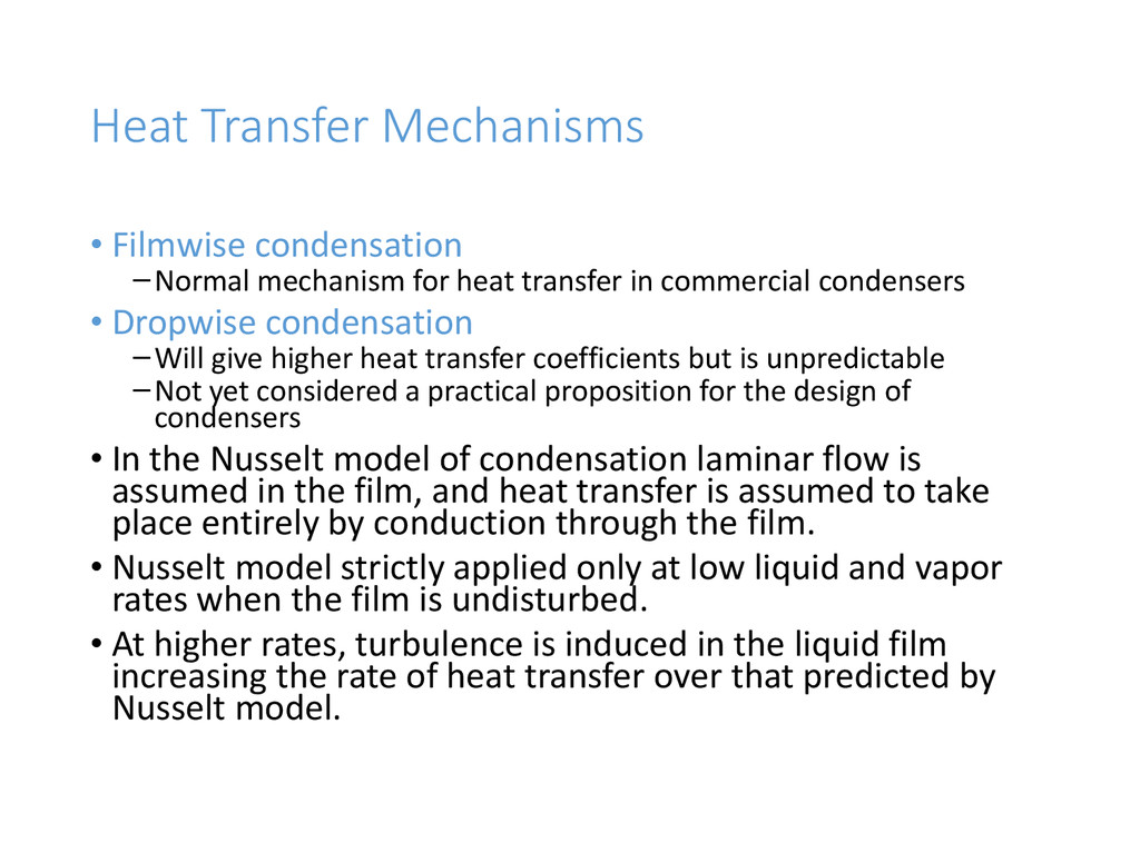
76. Heat Transfer Mechanisms • Filmwise condensation –Normal mechanism for heat transfer in commercial condensers • Dropwise condensation –Will give higher heat transfer coefficients but is unpredictable –Not yet considered a practical proposition for the design of condensers • In the Nusselt model of condensation laminar flow is assumed in the film, and heat transfer is assumed to take place entirely by conduction through the film. • Nusselt model strictly applied only at low liquid and vapor rates when the film is undisturbed. • At higher rates, turbulence is induced in the liquid film increasing the rate of heat transfer over that predicted by Nusselt model.
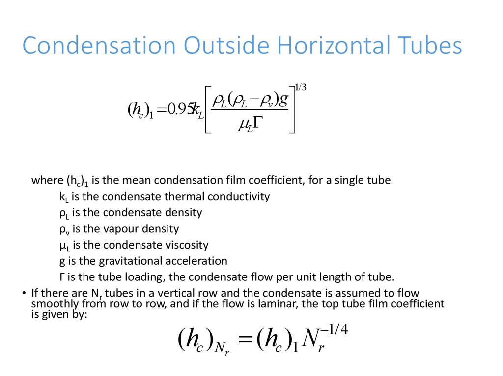
77. Condensation Outside Horizontal Tubes where (hc )1 is the mean condensation film coefficient, for a single tube kL is the condensate thermal conductivity ρL is the condensate density ρv is the vapour density μL is the condensate viscosity g is the gravitational acceleration Γ is the tube loading, the condensate flow per unit length of tube. • If there are Nr tubes in a vertical row and the condensate is assumed to flow smoothly from row to row, and if the flow is laminar, the top tube film coefficient is given by: 3 / 1 1 ) ( 95 . 0 ) (          L v L L L c g k h     4 / 1 1 ) ( ) (   r c N c N h h r
78. •
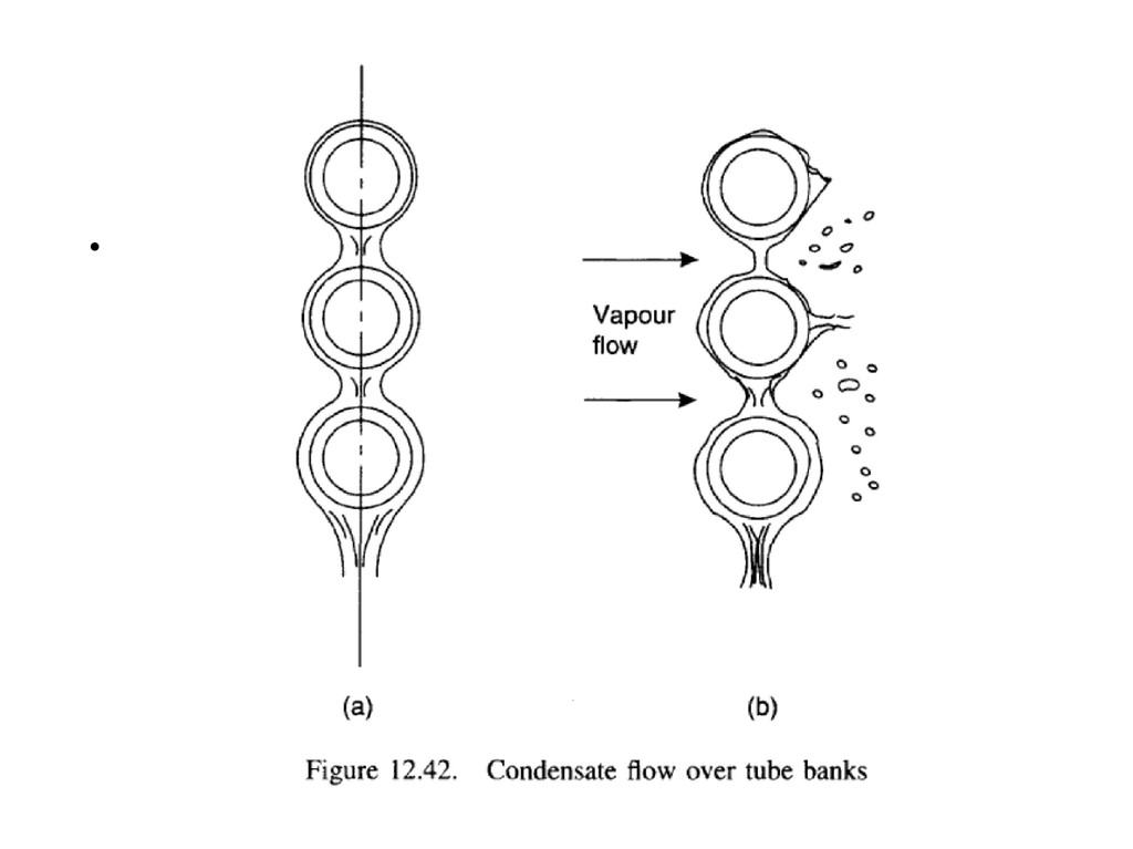
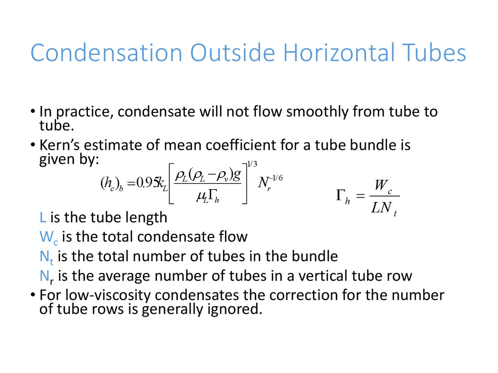
79. Condensation Outside Horizontal Tubes • In practice, condensate will not flow smoothly from tube to tube. • Kern’s estimate of mean coefficient for a tube bundle is given by: L is the tube length Wc is the total condensate flow Nt is the total number of tubes in the bundle Nr is the average number of tubes in a vertical tube row • For low-viscosity condensates the correction for the number of tube rows is generally ignored. 6 / 1 3 / 1 ) ( 95 . 0 ) (           r h L v L L L b c N g k h     t c h LN W  
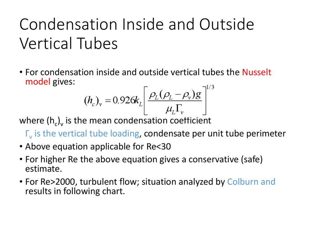
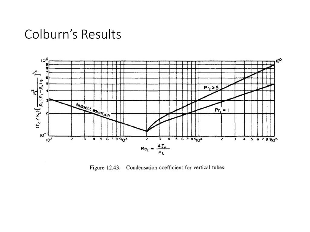
80. Condensation Inside and Outside Vertical Tubes • For condensation inside and outside vertical tubes the Nusselt model gives: where (hc )v is the mean condensation coefficient Γv is the vertical tube loading, condensate per unit tube perimeter • Above equation applicable for Re<30 • For higher Re the above equation gives a conservative (safe) estimate. • For Re>2000, turbulent flow; situation analyzed by Colburn and results in following chart. 3 / 1 ) ( 926 . 0 ) (          v L v L L L v c g k h    
81. Colburn’s Results
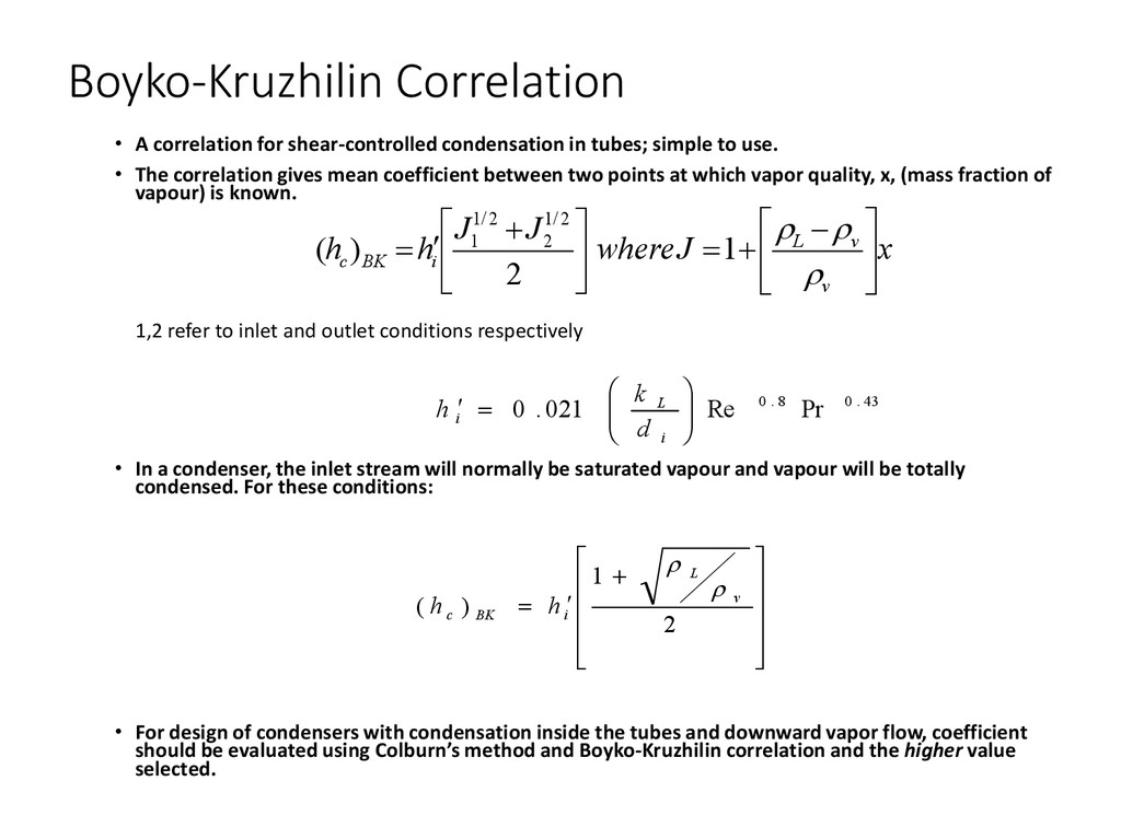
82. Boyko-Kruzhilin Correlation • A correlation for shear-controlled condensation in tubes; simple to use. • The correlation gives mean coefficient between two points at which vapor quality, x, (mass fraction of vapour) is known. 1,2 refer to inlet and outlet conditions respectively • In a condenser, the inlet stream will normally be saturated vapour and vapour will be totally condensed. For these conditions: • For design of condensers with condensation inside the tubes and downward vapor flow, coefficient should be evaluated using Colburn’s method and Boyko-Kruzhilin correlation and the higher value selected. x J where J J h h v v L i BK c                      1 2 ) ( 2 / 1 2 2 / 1 1 43 . 0 8 . 0 Pr Re 021 . 0           i L i d k h                2 1 ) ( v L i BK c h h  
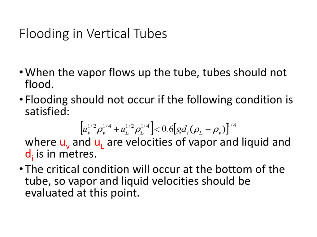
83. Flooding in Vertical Tubes •When the vapor flows up the tube, tubes should not flood. •Flooding should not occur if the following condition is satisfied: where uv and uL are velocities of vapor and liquid and di is in metres. •The critical condition will occur at the bottom of the tube, so vapor and liquid velocities should be evaluated at this point.     4 / 1 4 / 1 2 / 1 4 / 1 2 / 1 ) ( 6 . 0 v L i L L v v gd u u       
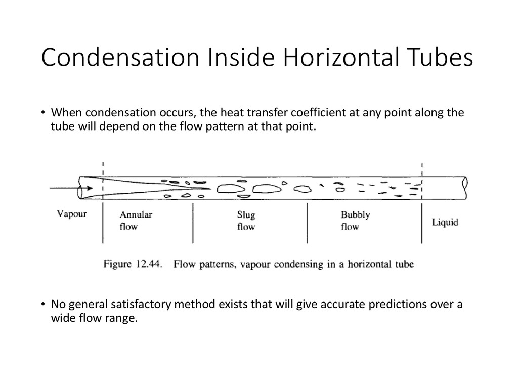
84. Condensation Inside Horizontal Tubes • When condensation occurs, the heat transfer coefficient at any point along the tube will depend on the flow pattern at that point. • No general satisfactory method exists that will give accurate predictions over a wide flow range.
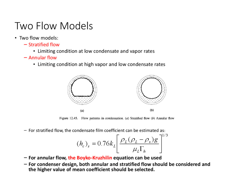
85. Two Flow Models • Two flow models: – Stratified flow • Limiting condition at low condensate and vapor rates – Annular flow • Limiting condition at high vapor and low condensate rates – For stratified flow, the condensate film coefficient can be estimated as: – For annular flow, the Boyko-Kruzhilin equation can be used – For condenser design, both annular and stratified flow should be considered and the higher value of mean coefficient should be selected. 3 / 1 ) ( 76 . 0 ) (          h L v L L L s c g k h    
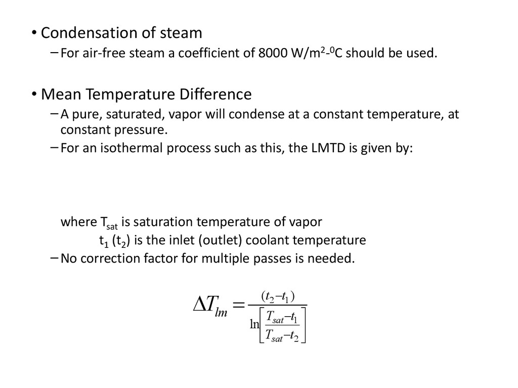
86. • Condensation of steam –For air-free steam a coefficient of 8000 W/m2-0C should be used. • Mean Temperature Difference –A pure, saturated, vapor will condense at a constant temperature, at constant pressure. –For an isothermal process such as this, the LMTD is given by: where Tsat is saturation temperature of vapor t1 (t2 ) is the inlet (outlet) coolant temperature –No correction factor for multiple passes is needed.            2 1 1 2 ln ) ( t T t T t t lm sat sat T