The Geometry of Efficient Training From Optimization History to Trajectory and Optimizer Geometry

https://www.ist.i.kyoto-u.ac.jp/news/2026/07/02/1676/

Transcript

1. The Geometry of Efficient Training From Optimization History to Trajectory and Optimizer Geometry Hiroki Naganuma Mila, Université de Montréal Intelligence Science and Technology Colloquium, Kyoto University Invited Talk / 2026 Geometry as a unifying lens for efficient optimization
2. TALK OVERVIEW | FIVE CHAPTERS Today’s Route 1 Foundations From empirical risk to stochastic gradients, smoothness, and preconditioning. 2 Field Map and Muon How scale changed optimizer design, and where spectral updates fit. 3 No Wrong Turns When a noisy update still follows a useful training direction. 4 Non-Euclidean GNS Critical batch size measured in the optimizer’s own geometry. 5 Decisions and Outlook A practical diagnostic workflow and open research questions. Hiroki Naganuma | Geometry of Efficient Training 2 / 49
3. CHAPTER 1 OF 5 Foundations What problem are we solving?
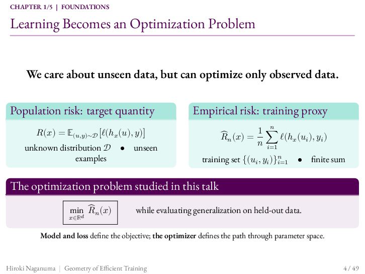
4. CHAPTER 1/5 | FOUNDATIONS Learning Becomes an Optimization Problem We care about unseen data, but can optimize only observed data. Population risk: target quantity Empirical risk: training proxy 𝑛 ̂𝑛 (𝑥) = 1 ∑ ℓ(ℎ𝑥 (𝑢𝑖 ), 𝑦𝑖 ) 𝑅 𝑛 𝑖=1 𝑅(𝑥) = 𝔼(𝑢,𝑦)∼𝒟 [ℓ(ℎ𝑥 (𝑢), 𝑦)] unknown distribution 𝒟 • examples unseen training set {(𝑢𝑖 , 𝑦𝑖 )}𝑛𝑖=1 • finite sum The optimization problem studied in this talk ̂𝑛 (𝑥) min 𝑅 𝑥∈ℝ𝑑 while evaluating generalization on held-out data. Model and loss define the objective; the optimizer defines the path through parameter space. Hiroki Naganuma | Geometry of Efficient Training 4 / 49
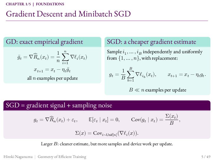
5. CHAPTER 1/5 | FOUNDATIONS Gradient Descent and Minibatch SGD GD: exact empirical gradient ̂𝑛 (𝑥𝑡 ) = 𝑔𝑡̄ = ∇𝑅 1 𝑛 ∑ ∇ℓ𝑖 (𝑥𝑡 ) 𝑛 𝑖=1 𝑥𝑡+1 = 𝑥𝑡 − 𝜂𝑡 𝑔𝑡̄ all 𝑛 examples per update SGD: a cheaper gradient estimate Sample 𝑖1 , … , 𝑖𝐵 independently and uniformly from {1, … , 𝑛}, with replacement: 𝑔𝑡 = 1 𝐵 ∑ ∇ℓ𝑖𝑏 (𝑥𝑡 ), 𝐵 𝑏=1 𝑥𝑡+1 = 𝑥𝑡 − 𝜂𝑡 𝑔𝑡 . 𝐵 ≪ 𝑛 examples per update SGD = gradient signal + sampling noise ̂𝑛 (𝑥𝑡 ) + 𝜀𝑡 , 𝑔𝑡 = ∇ 𝑅 𝔼[𝜀𝑡 ∣ 𝑥𝑡 ] = 0, Cov(𝑔𝑡 ∣ 𝑥𝑡 ) = Σ(𝑥𝑡 ) , 𝐵 Σ(𝑥) = Cov𝑖∼Unif[𝑛] (∇ℓ𝑖 (𝑥)). Larger 𝐵: cleaner estimate, but more samples and device work per update. Hiroki Naganuma | Geometry of Efficient Training 5 / 49
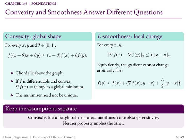
6. CHAPTER 1/5 | FOUNDATIONS Convexity and Smoothness Answer Different Questions Convexity: global shape 𝐿-smoothness: local change For every 𝑥, 𝑦 and 𝜃 ∈ [0, 1], For every 𝑥, 𝑦, 𝑓((1 − 𝜃)𝑥 + 𝜃𝑦) ≤ (1 − 𝜃)𝑓(𝑥) + 𝜃𝑓(𝑦). Chords lie above the graph. If 𝑓 is differentiable and convex, ∇𝑓(𝑥) = 0 implies a global minimum. ‖∇𝑓(𝑥) − ∇𝑓(𝑦)‖2 ≤ 𝐿‖𝑥 − 𝑦‖2 . Equivalently, the gradient cannot change arbitrarily fast: 𝑓(𝑦) ≤ 𝑓(𝑥) + ⟨∇𝑓(𝑥), 𝑦 − 𝑥⟩ + 𝐿 ‖𝑦 − 𝑥‖22 . 2 The minimizer need not be unique. Keep the assumptions separate Convexity identifies global structure; smoothness controls step sensitivity. Neither property implies the other. Hiroki Naganuma | Geometry of Efficient Training 6 / 49
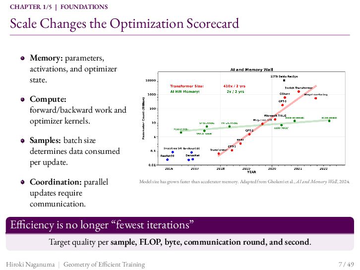
7. CHAPTER 1/5 | FOUNDATIONS Scale Changes the Optimization Scorecard Memory: parameters, activations, and optimizer state. Compute: forward/backward work and optimizer kernels. Samples: batch size determines data consumed per update. Coordination: parallel updates require communication. Model size has grown faster than accelerator memory. Adapted from Gholami et al., AI and Memory Wall, 2024. Efficiency is no longer “fewest iterations” Target quality per sample, FLOP, byte, communication round, and second. Hiroki Naganuma | Geometry of Efficient Training 7 / 49
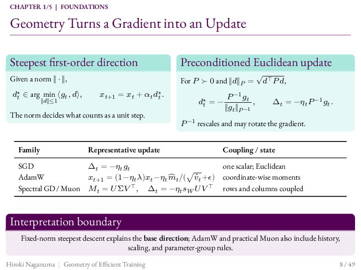
8. CHAPTER 1/5 | FOUNDATIONS Geometry Turns a Gradient into an Update Steepest first-order direction Preconditioned Euclidean update Given a norm ‖ ⋅ ‖, For 𝑃 ≻ 0 and ‖𝑑‖𝑃 = 𝑑𝑡⋆ ∈ arg min ⟨𝑔𝑡 , 𝑑⟩, ‖𝑑‖≤1 𝑥𝑡+1 = 𝑥𝑡 + 𝛼𝑡 𝑑𝑡⋆ . The norm decides what counts as a unit step. 𝑑𝑡⋆ = − 𝑃 −1 𝑔𝑡 , ‖𝑔𝑡 ‖𝑃 −1 √ 𝑑⊤ 𝑃 𝑑, Δ𝑡 = −𝜂𝑡 𝑃 −1 𝑔𝑡 . 𝑃 −1 rescales and may rotate the gradient. Family Representative update Coupling / state SGD AdamW Spectral GD / Muon Δ𝑡 = −𝜂𝑡 𝑔𝑡 𝑥𝑡+1 = (1−𝜂𝑡 𝜆)𝑥𝑡 −𝜂𝑡 𝑚 ̂ 𝑡 /(√𝑣𝑡̂ +𝜖) 𝑀𝑡 = 𝑈Σ𝑉 ⊤ , Δ𝑡 = −𝜂𝑡 𝑠𝑊 𝑈𝑉 ⊤ one scalar; Euclidean coordinate-wise moments rows and columns coupled Interpretation boundary Fixed-norm steepest descent explains the base direction; AdamW and practical Muon also include history, scaling, and parameter-group rules. Hiroki Naganuma | Geometry of Efficient Training 8 / 49
9. CHAPTER 2 OF 5 Field Map and Muon How optimizer design reached spectral updates
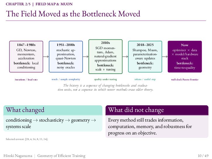
10. CHAPTER 2/5 | FIELD MAP & MUON The Field Moved as the Bottleneck Moved 1847–1980s GD, Newton, momentum, acceleration bottleneck: local conditioning 1951–2000s stochastic approximation, quasi-Newton bottleneck: noisy oracles 2010s SGD momentum, Adam, natural-gradient approximations bottleneck: scale + tuning 2018–2025 Shampoo, Muon, parameterizationaware updates bottleneck: geometry Now optimizer × data × model/hardware stack bottleneck: time-to-quality iterations / local rate oracle / sample complexity quality under tuning tokens / useful step wall-clock Pareto frontier The history is a sequence of changing bottlenecks and evaluation units, not a sequence in which newer methods erase older theory. What changed What did not change conditioning → stochasticity → geometry → systems scale Every method still trades information, computation, memory, and robustness for progress on an objective. Selected context: [28, 4, 16, 8, 11, 14]. Hiroki Naganuma | Geometry of Efficient Training 10 / 49
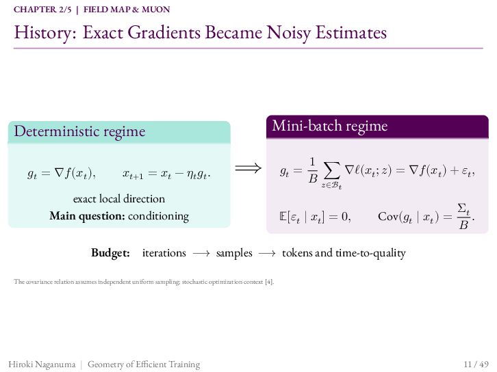
11. CHAPTER 2/5 | FIELD MAP & MUON History: Exact Gradients Became Noisy Estimates Mini-batch regime Deterministic regime 𝑔𝑡 = ∇𝑓(𝑥𝑡 ), 𝑥𝑡+1 = 𝑥𝑡 − 𝜂𝑡 𝑔𝑡 . ⟹ exact local direction Main question: conditioning Budget: 𝑔𝑡 = 1 ∑ ∇ℓ(𝑥𝑡 ; 𝑧) = ∇𝑓(𝑥𝑡 ) + 𝜀𝑡 , 𝐵 𝑧∈ℬ 𝑡 𝔼[𝜀𝑡 ∣ 𝑥𝑡 ] = 0, Cov(𝑔𝑡 ∣ 𝑥𝑡 ) = Σ𝑡 . 𝐵 iterations ⟶ samples ⟶ tokens and time-to-quality The covariance relation assumes independent uniform sampling; stochastic optimization context [4]. Hiroki Naganuma | Geometry of Efficient Training 11 / 49
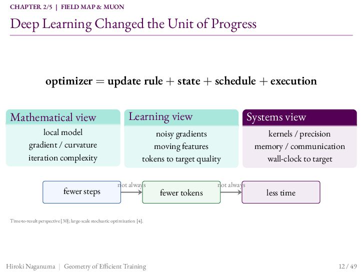
12. CHAPTER 2/5 | FIELD MAP & MUON Deep Learning Changed the Unit of Progress optimizer = update rule + state + schedule + execution Mathematical view local model gradient / curvature iteration complexity fewer steps Learning view Systems view noisy gradients moving features tokens to target quality not always fewer tokens not always kernels / precision memory / communication wall-clock to target less time Time-to-result perspective [30]; large-scale stochastic optimization [4]. Hiroki Naganuma | Geometry of Efficient Training 12 / 49
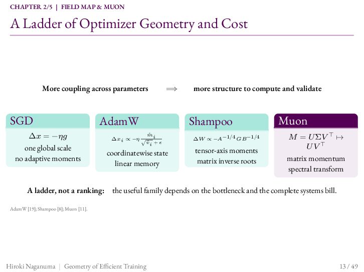
13. CHAPTER 2/5 | FIELD MAP & MUON A Ladder of Optimizer Geometry and Cost More coupling across parameters SGD ⟹ AdamW Δ𝑥 = −𝜂𝑔 one global scale no adaptive moments A ladder, not a ranking: 𝑚̂ 𝑖 Δ𝑥𝑖 ∝ −𝜂 √𝑣̂ 𝑖 + 𝜖 coordinatewise state linear memory more structure to compute and validate Shampoo Δ𝑊 ∝ −𝐴−1/4 𝐺𝐵−1/4 tensor-axis moments matrix inverse roots Muon 𝑀 = 𝑈Σ𝑉 ⊤ ↦ 𝑈𝑉 ⊤ matrix momentum spectral transform the useful family depends on the bottleneck and the complete systems bill. AdamW [19]; Shampoo [8]; Muon [11]. Hiroki Naganuma | Geometry of Efficient Training 13 / 49
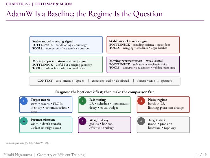
14. CHAPTER 2/5 | FIELD MAP & MUON AdamW Is a Baseline; the Regime Is the Question Stable model + strong signal Stable model + weak signal Moving representation + strong signal Moving representation + weak signal BOTTLENECK sampling variance / noise floor TOOLS averaging • schedules • larger batches BOTTLENECK conditioning / anisotropy TOOLS momentum • line search • curvature BOTTLENECK useful but changing geometry TOOLS robust first order • normalization CONTEXT data: stream ↔ epochs BOTTLENECK stale state + stochastic noise TOOLS conservative adaptation • validate extra state | execution: local ↔ distributed | objects: vectors ↔ operators Diagnose the bottleneck first; then make the comparison fair. 1 Target metric steps • tokens • FLOPs memory • communication • time 2 Fair tuning LR • schedule • momentum decay • equal budget 3 Noise regime batch × LR limiting phase can change 4 Parameterization width / depth transfer update-to-weight scale 5 Weight decay groups • horizon effective shrinkage 6 Target stack model • precision hardware • topology Fair comparisons [5, 25]; AdamW [19]. Hiroki Naganuma | Geometry of Efficient Training 14 / 49
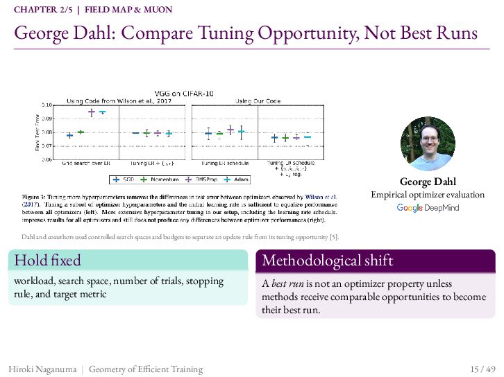
15. CHAPTER 2/5 | FIELD MAP & MUON George Dahl: Compare Tuning Opportunity, Not Best Runs George Dahl Empirical optimizer evaluation Dahl and coauthors used controlled search spaces and budgets to separate an update rule from its tuning opportunity [5]. Hold fixed Methodological shift workload, search space, number of trials, stopping rule, and target metric A best run is not an optimizer property unless methods receive comparable opportunities to become their best run. Hiroki Naganuma | Geometry of Efficient Training 15 / 49
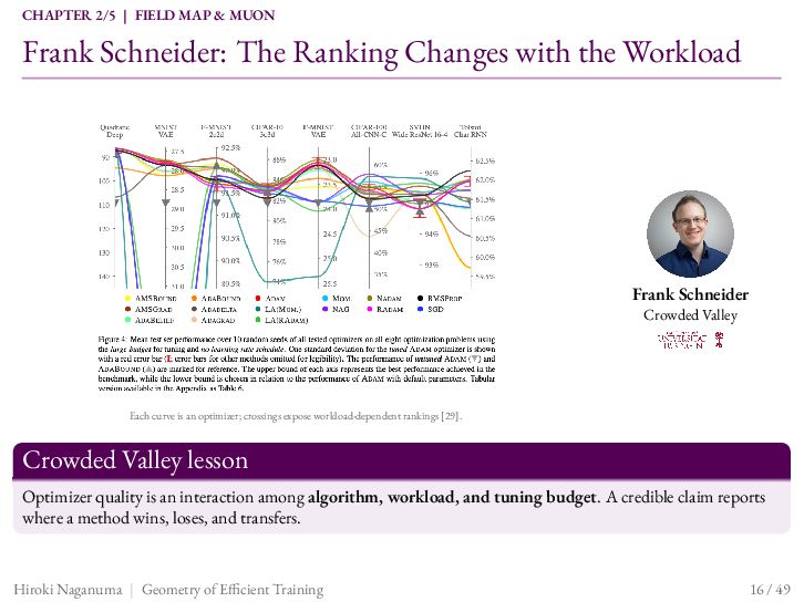
16. CHAPTER 2/5 | FIELD MAP & MUON Frank Schneider: The Ranking Changes with the Workload Frank Schneider Crowded Valley Each curve is an optimizer; crossings expose workload-dependent rankings [29]. Crowded Valley lesson Optimizer quality is an interaction among algorithm, workload, and tuning budget. A credible claim reports where a method wins, loses, and transfers. Hiroki Naganuma | Geometry of Efficient Training 16 / 49
17. CHAPTER 2/5 | FIELD MAP & MUON AlgoPerf Turned Those Lessons into a Protocol Workload suite models, data, targets, and implementations Tuning budget search space, trials, and validation rules External tuning: hyperparameters may be selected per workload within the common protocol. Ruleset external tuning or self-tuning submission Score time-to-target aggregated across workloads Self tuning: one submission must adapt without workload-specific manual tuning. The protocol turns “optimizer A won my run” into a testable claim. Scores from different rulesets are not directly comparable. George Dahl: comparable evaluation Frank Schneider: workload sensitivity Two rulesets answer two questions External tuning controls a workload-specific search budget; self tuning asks one submission to adapt without manual workload-specific search [14]. Hiroki Naganuma | Geometry of Efficient Training 17 / 49
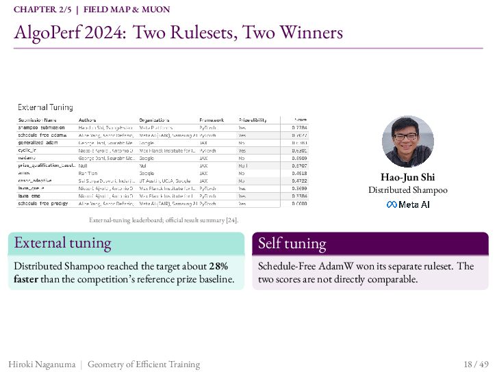
18. CHAPTER 2/5 | FIELD MAP & MUON AlgoPerf 2024: Two Rulesets, Two Winners Hao-Jun Shi Distributed Shampoo External-tuning leaderboard; official result summary [24]. External tuning Self tuning Distributed Shampoo reached the target about 28% faster than the competition’s reference prize baseline. Schedule-Free AdamW won its separate ruleset. The two scores are not directly comparable. Hiroki Naganuma | Geometry of Efficient Training 18 / 49
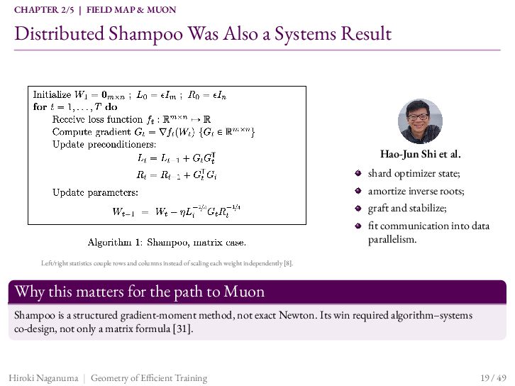
19. CHAPTER 2/5 | FIELD MAP & MUON Distributed Shampoo Was Also a Systems Result Hao-Jun Shi et al. shard optimizer state; amortize inverse roots; graft and stabilize; fit communication into data parallelism. Left/right statistics couple rows and columns instead of scaling each weight independently [8]. Why this matters for the path to Muon Shampoo is a structured gradient-moment method, not exact Newton. Its win required algorithm–systems co-design, not only a matrix formula [31]. Hiroki Naganuma | Geometry of Efficient Training 19 / 49
20. CHAPTER 2/5 | FIELD MAP & MUON Second Order: Different Objects, Different Systems Bills FAMILY MATHEMATICAL OBJECT COMPUTE / SYSTEMS BILL Exact Newton loss Hessian + linear solve 𝑝2 state • solve • damping/globalization; infeasible as an LLM default HF Newton / LBFGS Hessian/GGN products or secant history (distinct mechanisms) inner iterations or curvature pairs • preconditioning • synchronization Natural gradient / K-FAC Fisher metric; K-FAC uses Kroneckerfactored blocks factor statistics • inverses • damping • memory / communication Shampoo accumulated gradient second moments + matrix inverse roots matrix statistics / roots • damping • sharding • memory traffic Muon momentum + approximate orthogonalization; spectral first-order update matrix functions • kernels • shape scaling • parameter-group rules Why exact Newton is not the LLM default The saved steps must repay dense curvature state, solves, damping, memory traffic, and synchronization. Structured approximations can still win when that balance is favorable. Terminology guardrail: Newton optimizes a Hessian-based local model; Newton–Schulz below is only a matrix-function iteration. Hessian-free optimization [20]; K-FAC [21]; Shampoo [8]. Hiroki Naganuma | Geometry of Efficient Training 20 / 49
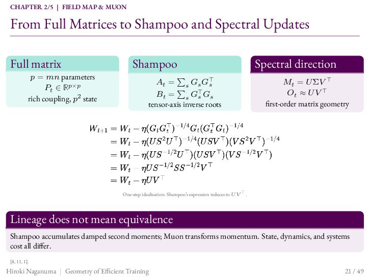
21. CHAPTER 2/5 | FIELD MAP & MUON From Full Matrices to Shampoo and Spectral Updates Full matrix 𝑝 = 𝑚𝑛 parameters 𝑃𝑡 ∈ ℝ𝑝×𝑝 rich coupling, 𝑝2 state Shampoo 𝐴𝑡 = ∑𝑠 𝐺𝑠 𝐺⊤ 𝑠 𝐵𝑡 = ∑𝑠 𝐺⊤ 𝑠 𝐺𝑠 tensor-axis inverse roots Spectral direction 𝑀𝑡 = 𝑈Σ𝑉 ⊤ 𝑂𝑡 ≈ 𝑈𝑉 ⊤ first-order matrix geometry One-step idealization: Shampoo’s expression reduces to 𝑈𝑉 ⊤ . Lineage does not mean equivalence Shampoo accumulates damped second moments; Muon transforms momentum. State, dynamics, and systems cost all differ. [8, 11, 1]. Hiroki Naganuma | Geometry of Efficient Training 21 / 49
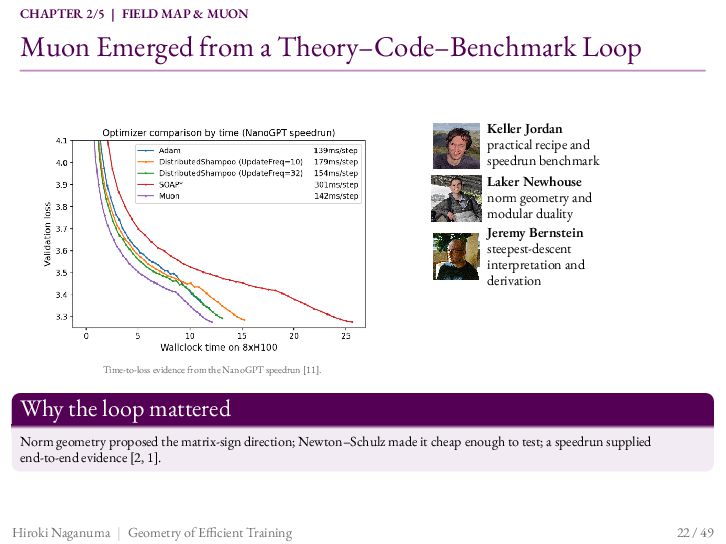
22. CHAPTER 2/5 | FIELD MAP & MUON Muon Emerged from a Theory–Code–Benchmark Loop Keller Jordan practical recipe and speedrun benchmark Laker Newhouse norm geometry and modular duality Jeremy Bernstein steepest-descent interpretation and derivation Time-to-loss evidence from the NanoGPT speedrun [11]. Why the loop mattered Norm geometry proposed the matrix-sign direction; Newton–Schulz made it cheap enough to test; a speedrun supplied end-to-end evidence [2, 1]. Hiroki Naganuma | Geometry of Efficient Training 22 / 49
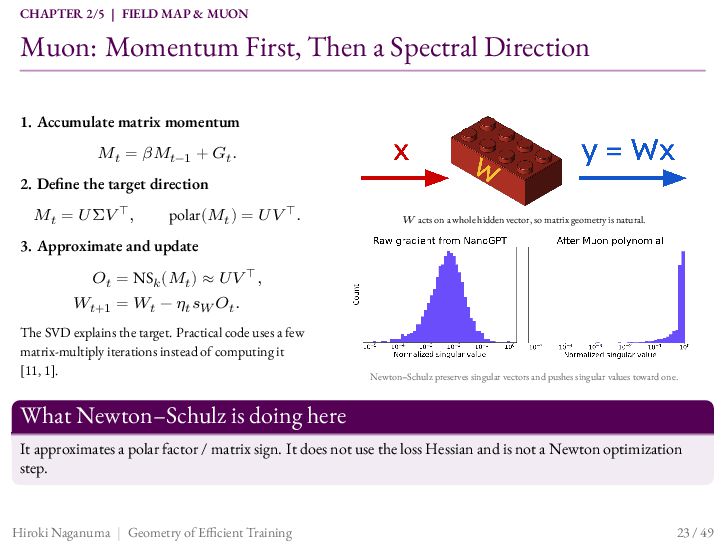
23. CHAPTER 2/5 | FIELD MAP & MUON Muon: Momentum First, Then a Spectral Direction 1. Accumulate matrix momentum 𝑀𝑡 = 𝛽𝑀𝑡−1 + 𝐺𝑡 . 2. Define the target direction 𝑀𝑡 = 𝑈Σ𝑉 ⊤ , polar(𝑀𝑡 ) = 𝑈𝑉 ⊤ . 𝑊 acts on a whole hidden vector, so matrix geometry is natural. 3. Approximate and update 𝑂𝑡 = NS𝑘 (𝑀𝑡 ) ≈ 𝑈𝑉 ⊤ , 𝑊𝑡+1 = 𝑊𝑡 − 𝜂𝑡 𝑠𝑊 𝑂𝑡 . The SVD explains the target. Practical code uses a few matrix-multiply iterations instead of computing it [11, 1]. Newton–Schulz preserves singular vectors and pushes singular values toward one. What Newton–Schulz is doing here It approximates a polar factor / matrix sign. It does not use the loss Hessian and is not a Newton optimization step. Hiroki Naganuma | Geometry of Efficient Training 23 / 49
24. CHAPTER 3 OF 5 No Wrong Turns When noisy steps still make progress
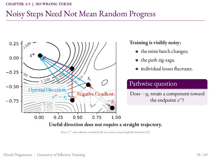
25. CHAPTER 3/5 | NO WRONG TURNS Noisy Steps Need Not Mean Random Progress Training is visibly noisy: the mini-batch changes; the path zig-zags; individual losses fluctuate. Pathwise question Does −𝑔𝑡 retain a component toward the endpoint 𝑥⋆ ? Useful direction does not require a straight trajectory. Here 𝑥⋆ is the solution reached by the run, not an assumed global minimizer [7]. Hiroki Naganuma | Geometry of Efficient Training 25 / 49
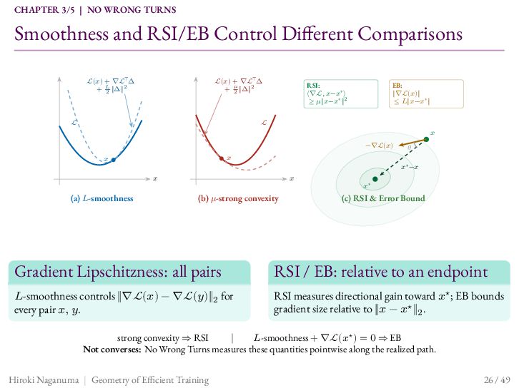
26. CHAPTER 3/5 | NO WRONG TURNS Smoothness and RSI/EB Control Different Comparisons ℒ(𝑥) + ∇ℒ⊤Δ 2 + 𝐿 2 ‖Δ‖ ℒ(𝑥) + ∇ℒ⊤Δ 2 + 𝜇 2 ‖Δ‖ ℒ EB: ‖∇ℒ(𝑥)‖ ≤ 𝐿‖𝑥−𝑥∗ ‖ RSI: ⟨∇ℒ, 𝑥−𝑥∗ ⟩ ≥ 𝜇‖𝑥−𝑥∗ ‖2 ℒ 𝑥 −∇ℒ(𝑥) 𝜃 𝑥 𝑥 𝑥∗ −𝑥 𝑥 𝑥 ∗ 𝑥 (a) 𝐿-smoothness (b) 𝜇-strong convexity (c) RSI & Error Bound Gradient Lipschitzness: all pairs RSI / EB: relative to an endpoint 𝐿-smoothness controls ‖∇ℒ(𝑥) − ∇ℒ(𝑦)‖2 for every pair 𝑥, 𝑦. RSI measures directional gain toward 𝑥⋆ ; EB bounds gradient size relative to ‖𝑥 − 𝑥⋆ ‖2 . strong convexity ⇒ RSI | 𝐿-smoothness + ∇ℒ(𝑥⋆ ) = 0 ⇒ EB Not converses: No Wrong Turns measures these quantities pointwise along the realized path. Hiroki Naganuma | Geometry of Efficient Training 26 / 49
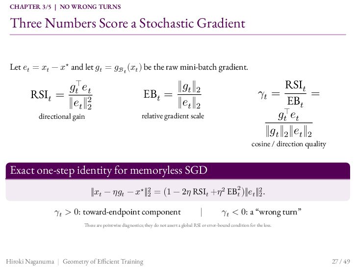
27. CHAPTER 3/5 | NO WRONG TURNS Three Numbers Score a Stochastic Gradient Let 𝑒𝑡 = 𝑥𝑡 − 𝑥⋆ and let 𝑔𝑡 = 𝑔ℬ𝑡 (𝑥𝑡 ) be the raw mini-batch gradient. 𝑔𝑡⊤ 𝑒𝑡 RSI𝑡 = ‖𝑒𝑡 ‖22 directional gain EB𝑡 = ‖𝑔𝑡 ‖2 ‖𝑒𝑡 ‖2 RSI𝑡 = EB𝑡 𝑔𝑡⊤ 𝑒𝑡 ‖𝑔𝑡 ‖2 ‖𝑒𝑡 ‖2 𝛾𝑡 = relative gradient scale cosine / direction quality Exact one-step identity for memoryless SGD ‖𝑥𝑡 − 𝜂𝑔𝑡 − 𝑥⋆ ‖22 = (1 − 2𝜂 RSI𝑡 +𝜂2 EB2𝑡 )‖𝑒𝑡 ‖22 . 𝛾𝑡 > 0: toward-endpoint component | 𝛾𝑡 < 0: a “wrong turn” These are pointwise diagnostics; they do not assert a global RSI or error-bound condition for the loss. Hiroki Naganuma | Geometry of Efficient Training 27 / 49
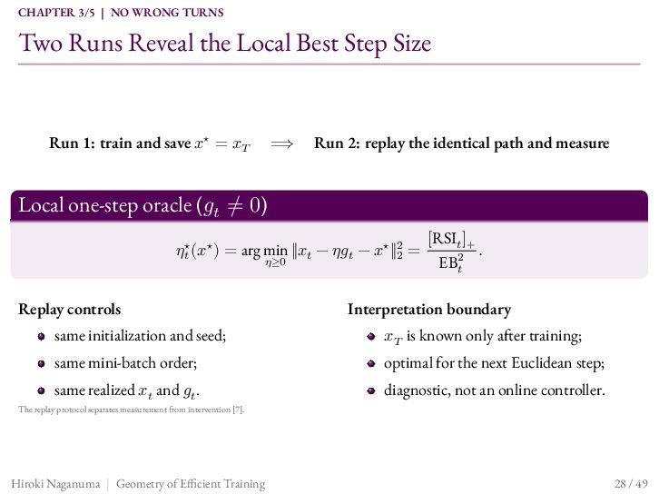
28. CHAPTER 3/5 | NO WRONG TURNS Two Runs Reveal the Local Best Step Size Run 1: train and save 𝑥⋆ = 𝑥𝑇 ⟹ Run 2: replay the identical path and measure Local one-step oracle (𝑔𝑡 ≠ 0) 𝜂𝑡⋆ (𝑥⋆ ) = arg min ‖𝑥𝑡 − 𝜂𝑔𝑡 − 𝑥⋆ ‖22 = 𝜂≥0 Replay controls [RSI𝑡 ]+ EB2𝑡 . Interpretation boundary same initialization and seed; 𝑥𝑇 is known only after training; same mini-batch order; optimal for the next Euclidean step; same realized 𝑥𝑡 and 𝑔𝑡 . diagnostic, not an online controller. The replay protocol separates measurement from intervention [7]. Hiroki Naganuma | Geometry of Efficient Training 28 / 49
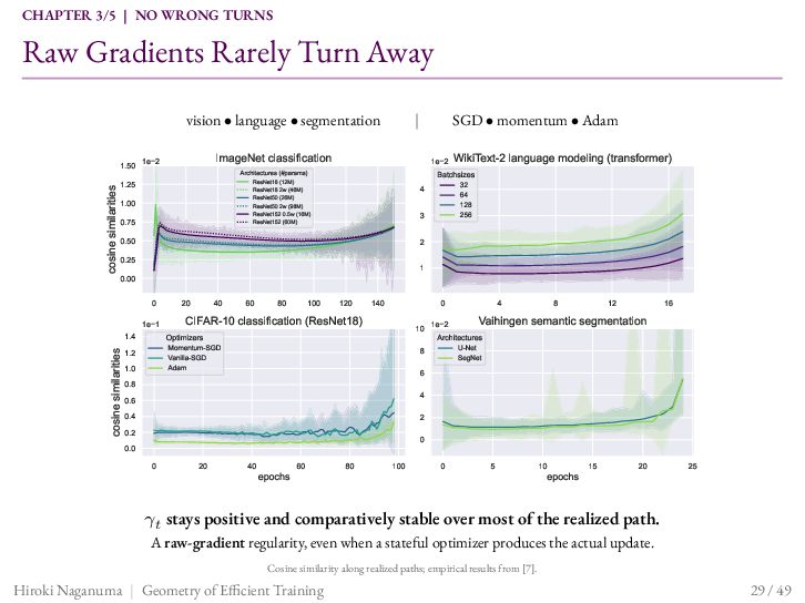
29. CHAPTER 3/5 | NO WRONG TURNS Raw Gradients Rarely Turn Away vision • language • segmentation ImageNet classification cosine similarities 1.50 1e 2 1e 2 WikiText-2 language modeling (transformer) Batchsizes Architectures (#params) ResNet18 (12M) ResNet18 2w (46M) ResNet50 (26M) ResNet50 2w (98M) ResNet152 0.5w (16M) ResNet152 (60M) 1.25 1.00 0.75 32 64 128 256 4 3 0.50 2 0.25 1 0.00 0 1e 1 cosine similarities SGD • momentum • Adam | 1.4 1.2 1.0 0.8 0.6 0.4 0.2 0.0 20 40 60 80 100 120 140 0 CIFAR-10 classification (ResNet18) 4 8 12 16 Vaihingen semantic segmentation 10 1e 2 Architectures U-Net 8 Optimizers Momentum-SGD Vanilla-SGD Adam SegNet 6 4 2 0 0 20 40 epochs 60 80 100 0 5 10 epochs 15 20 25 𝛾𝑡 stays positive and comparatively stable over most of the realized path. A raw-gradient regularity, even when a stateful optimizer produces the actual update. Cosine similarity along realized paths; empirical results from [7]. Hiroki Naganuma | Geometry of Efficient Training 29 / 49
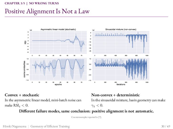
30. CHAPTER 3/5 | NO WRONG TURNS Positive Alignment Is Not a Law 6 Asymmetric linear model (stochastic) 1e3 0 RSI 2 5 0 10 2 15 4 20 6 25 8 0 cosine similarities Sinusoidal mixture (non-convex) 1e2 5 4 10 20 30 40 50 60 70 1.0 1.0 0.5 0.5 0.0 0.0 0.5 0.5 1.0 0 10 20 30 40 epochs 50 Convex + stochastic 60 70 In the asymmetric linear model, mini-batch noise can make RSI𝑡 < 0. 1.0 0 200 400 600 800 1000 0 200 400 600 800 1000 iterations Non-convex + deterministic In the sinusoidal mixture, basin geometry can make 𝛾𝑡 < 0. Different failure modes, same conclusion: positive alignment is not automatic. Counterexamples reported in [7]. Hiroki Naganuma | Geometry of Efficient Training 30 / 49
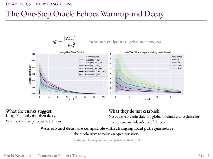
31. CHAPTER 3/5 | NO WRONG TURNS The One-Step Oracle Echoes Warmup and Decay 𝜂𝑡⋆ = [RSI𝑡 ]+ ImageNet Classification 0.30 0.20 0.15 WikiText-2 Language Modeling (transformer) 8 Architectures ResNet18 (12M) ResNet18 2w (46M) ResNet50 (26M) ResNet50 2w (98M) ResNet152 0.5w (16M) ResNet152 (60M) 0.25 Locally optimal LR post-hoc, endpoint-relative, memoryless EB2𝑡 Batchsizes 7 32 64 128 256 6 5 4 3 0.10 2 0.05 1 0 0.00 0 25 50 75 100 epochs 125 What the curves suggest 150 175 0 4 8 epochs 12 16 What they do not establish ImageNet: early rise, then decay. WikiText-2: decay across batch sizes. No deployable schedule; no global optimality; no claim for momentum or Adam’s stateful update. Warmup and decay are compatible with changing local path geometry; the mechanism remains an open question. The displayed learning rates were computed after the runs [7]. Hiroki Naganuma | Geometry of Efficient Training 31 / 49
32. CHAPTER 4 OF 5 Non-Euclidean GNS Batch-size scaling in the optimizer’s geometry
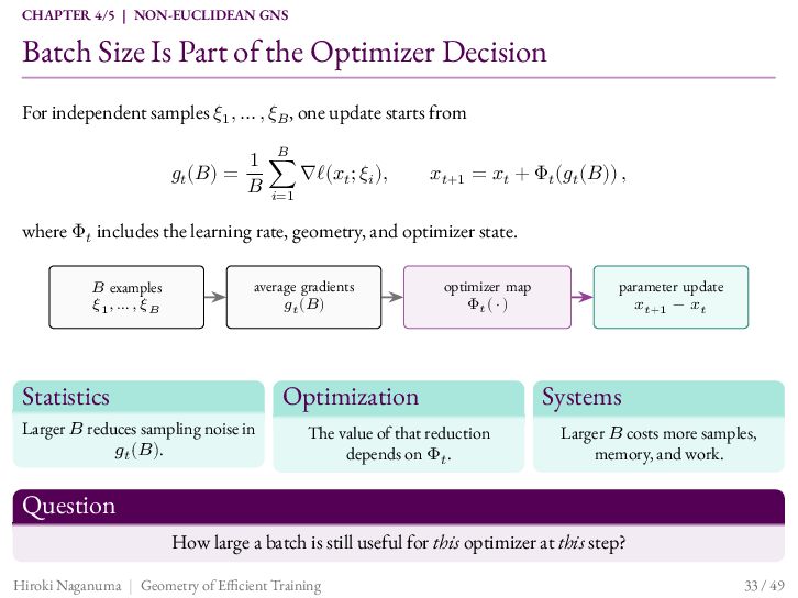
33. CHAPTER 4/5 | NON-EUCLIDEAN GNS Batch Size Is Part of the Optimizer Decision For independent samples 𝜉1 , … , 𝜉𝐵 , one update starts from 𝑔𝑡 (𝐵) = 1 𝐵 ∑ ∇ℓ(𝑥𝑡 ; 𝜉𝑖 ), 𝐵 𝑖=1 𝑥𝑡+1 = 𝑥𝑡 + Φ𝑡 (𝑔𝑡 (𝐵)) , where Φ𝑡 includes the learning rate, geometry, and optimizer state. 𝐵 examples 𝜉1 , … , 𝜉𝐵 average gradients 𝑔𝑡 (𝐵) Statistics optimizer map Φ𝑡 ( ⋅ ) Optimization Larger 𝐵 reduces sampling noise in 𝑔𝑡 (𝐵). The value of that reduction depends on Φ𝑡 . parameter update 𝑥𝑡+1 − 𝑥𝑡 Systems Larger 𝐵 costs more samples, memory, and work. Question How large a batch is still useful for this optimizer at this step? Hiroki Naganuma | Geometry of Efficient Training 33 / 49
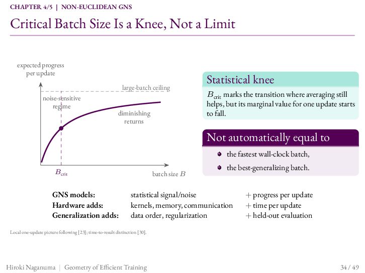
34. CHAPTER 4/5 | NON-EUCLIDEAN GNS Critical Batch Size Is a Knee, Not a Limit expected progress per update large-batch ceiling noise-sensitive regime diminishing returns Statistical knee 𝐵crit marks the transition where averaging still helps, but its marginal value for one update starts to fall. Not automatically equal to the fastest wall-clock batch, 𝐵crit GNS models: Hardware adds: Generalization adds: batch size 𝐵 the best-generalizing batch. statistical signal/noise kernels, memory, communication data order, regularization + progress per update + time per update + held-out evaluation Local one-update picture following [23]; time-to-result distinction [30]. Hiroki Naganuma | Geometry of Efficient Training 34 / 49
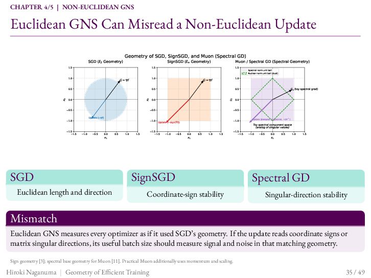
35. CHAPTER 4/5 | NON-EUCLIDEAN GNS Euclidean GNS Can Misread a Non-Euclidean Update SGD ( 2 Geometry) Geometry of SGD, SignSGD, and Muon (Spectral GD) SignSGD ( Geometry) 1.5 1.0 1.5 1.0 G= f 0.5 0.0 0.0 Update ( f) 1.0 1.5 1.5 1.0 0.5 0.0 x1 SGD Euclidean length and direction 0.5 1.0 1.5 s2 0.5 0.0 0.5 0.5 0.5 1.0 Update ( sign( f)) 1.0 1.5 1.5 1.5 1.0 0.5 0.0 x1 0.5 1.0 Spectral norm unit ball Nuclear norm unit ball (dual) 1.0 G= f 0.5 x2 x2 Muon / Spectral GD (Spectral Geometry) 1.5 1.5 SignSGD Coordinate-sign stability Gs (toy spectral grad) Update (steepest in spectral, UV ) Toy spectral component space (analog of singular values) 1.5 1.0 0.5 0.0 s1 0.5 1.0 1.5 Spectral GD Singular-direction stability Mismatch Euclidean GNS measures every optimizer as if it used SGD’s geometry. If the update reads coordinate signs or matrix singular directions, its useful batch size should measure signal and noise in that matching geometry. Sign geometry [3]; spectral base geometry for Muon [11]. Practical Muon additionally uses momentum and scaling. Hiroki Naganuma | Geometry of Efficient Training 35 / 49
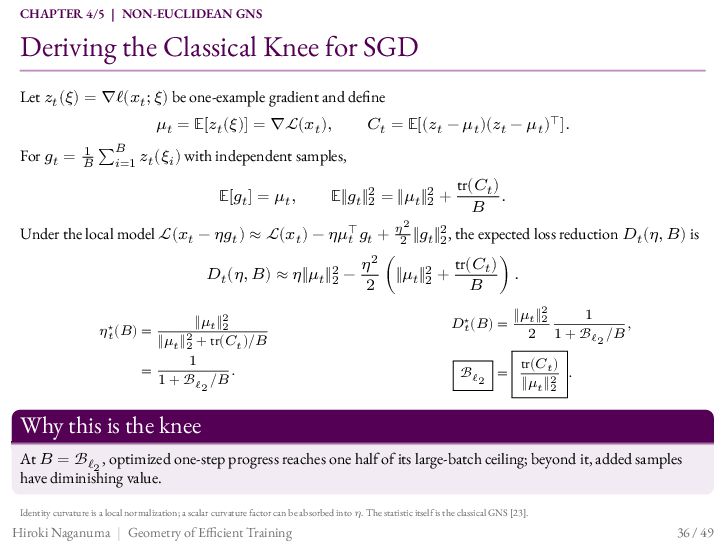
36. CHAPTER 4/5 | NON-EUCLIDEAN GNS Deriving the Classical Knee for SGD Let 𝑧𝑡 (𝜉) = ∇ℓ(𝑥𝑡 ; 𝜉) be one-example gradient and define 𝜇𝑡 = 𝔼[𝑧𝑡 (𝜉)] = ∇ℒ(𝑥𝑡 ), 𝐶𝑡 = 𝔼[(𝑧𝑡 − 𝜇𝑡 )(𝑧𝑡 − 𝜇𝑡 )⊤ ]. 𝐵 1 For 𝑔𝑡 = 𝐵 ∑𝑖=1 𝑧𝑡 (𝜉𝑖 ) with independent samples, 𝔼[𝑔𝑡 ] = 𝜇𝑡 , 𝔼‖𝑔𝑡 ‖22 = ‖𝜇𝑡 ‖22 + tr(𝐶𝑡 ) . 𝐵 2 𝜂 2 Under the local model ℒ(𝑥𝑡 − 𝜂𝑔𝑡 ) ≈ ℒ(𝑥𝑡 ) − 𝜂𝜇⊤ 𝑡 𝑔𝑡 + 2 ‖𝑔𝑡 ‖2 , the expected loss reduction 𝐷𝑡 (𝜂, 𝐵) is 𝐷𝑡 (𝜂, 𝐵) ≈ 𝜂‖𝜇𝑡 ‖22 − 𝜂𝑡⋆ (𝐵) = = ‖𝜇𝑡 ‖22 ‖𝜇𝑡 ‖22 + tr(𝐶𝑡 )/𝐵 1 . 1 + ℬℓ2 /𝐵 𝜂2 tr(𝐶𝑡 ) (‖𝜇𝑡 ‖22 + ). 2 𝐵 𝐷⋆𝑡 (𝐵) = ‖𝜇𝑡 ‖22 1 , 2 1 + ℬℓ2 /𝐵 ℬ ℓ2 = tr(𝐶𝑡 ) . ‖𝜇𝑡 ‖22 Why this is the knee At 𝐵 = ℬℓ2 , optimized one-step progress reaches one half of its large-batch ceiling; beyond it, added samples have diminishing value. Identity curvature is a local normalization; a scalar curvature factor can be absorbed into 𝜂. The statistic itself is the classical GNS [23]. Hiroki Naganuma | Geometry of Efficient Training 36 / 49
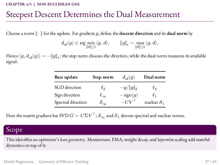
37. CHAPTER 4/5 | NON-EUCLIDEAN GNS Steepest Descent Determines the Dual Measurement Choose a norm ‖ ⋅ ‖ for the update. For gradient 𝑔, define the descent direction and its dual norm by 𝑑sd (𝑔) ∈ arg min ⟨𝑔, 𝑑⟩, ‖𝑑‖≤1 ‖𝑔‖⋆ = max ⟨𝑔, 𝑑⟩. ‖𝑑‖≤1 Hence ⟨𝑔, 𝑑sd (𝑔)⟩ = −‖𝑔‖⋆ : the step norm chooses the direction, while the dual norm measures its available signal. Base update Step norm 𝑑sd (𝑔) Dual norm SGD direction ℓ2 −𝑔/‖𝑔‖2 ℓ2 Sign direction ℓ∞ − sign(𝑔) ℓ1 Spectral direction 𝒮∞ −𝑈𝑉 ⊤ nuclear 𝒮1 Here the matrix gradient has SVD 𝐺 = 𝑈Σ𝑉 ⊤ ; 𝒮∞ and 𝒮1 denote spectral and nuclear norms. Scope This identifies an optimizer’s base geometry. Momentum, EMA, weight decay, and layerwise scaling add stateful dynamics on top of it. Hiroki Naganuma | Geometry of Efficient Training 37 / 49
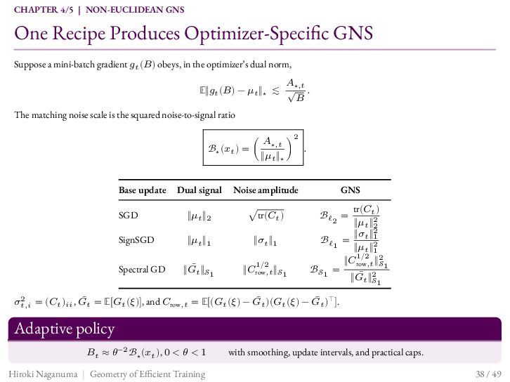
38. CHAPTER 4/5 | NON-EUCLIDEAN GNS One Recipe Produces Optimizer-Specific GNS Suppose a mini-batch gradient 𝑔𝑡 (𝐵) obeys, in the optimizer’s dual norm, 𝐴⋆,𝑡 𝔼‖𝑔𝑡 (𝐵) − 𝜇𝑡 ‖⋆ ≲ √ . 𝐵 The matching noise scale is the squared noise-to-signal ratio ℬ⋆ (𝑥𝑡 ) = ( Base update 𝐴⋆,𝑡 ) ‖𝜇𝑡 ‖⋆ 2 Dual signal Noise amplitude SGD ‖𝜇𝑡 ‖2 √tr(𝐶𝑡 ) SignSGD ‖𝜇𝑡 ‖1 ‖𝜎𝑡 ‖1 Spectral GD ‖𝐺𝑡̄ ‖𝒮1 ‖𝐶row,𝑡 ‖𝒮1 1/2 . GNS tr(𝐶𝑡 ) ‖𝜇𝑡 ‖22 ‖𝜎𝑡 ‖21 ℬℓ1 = ‖𝜇𝑡 ‖21 1/2 ‖𝐶row,𝑡 ‖2𝒮 1 ℬ𝒮1 = ‖𝐺 ̄ ‖2 ℬℓ2 = 𝑡 𝒮1 2 = (𝐶𝑡 )𝑖𝑖 , 𝐺𝑡̄ = 𝔼[𝐺𝑡 (𝜉)], and 𝐶row,𝑡 = 𝔼[(𝐺𝑡 (𝜉) − 𝐺𝑡̄ )(𝐺𝑡 (𝜉) − 𝐺𝑡̄ )⊤ ]. 𝜎𝑡,𝑖 Adaptive policy 𝐵𝑡 ≈ 𝜃−2 ℬ⋆ (𝑥𝑡 ), 0 < 𝜃 < 1 Hiroki Naganuma | Geometry of Efficient Training with smoothing, update intervals, and practical caps. 38 / 49
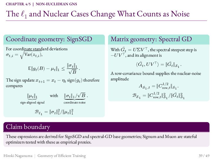
39. CHAPTER 4/5 | NON-EUCLIDEAN GNS The ℓ1 and Nuclear Cases Change What Counts as Noise Coordinate geometry: SignSGD Matrix geometry: Spectral GD For coordinate standard deviations 𝜎𝑡,𝑖 = √Var(𝑧𝑡,𝑖 ), With 𝐺𝑡̄ = 𝑈Σ𝑉 ⊤ , the spectral steepest step is −𝑈𝑉 ⊤ , and its alignment is ‖𝜎 ‖ 𝔼‖𝑔𝑡 (𝐵) − 𝜇𝑡 ‖1 ≤ √𝑡 1 . 𝐵 The sign update 𝑥𝑡+1 = 𝑥𝑡 − 𝜂𝑡 sign(𝑔𝑡 ) therefore compares √ ‖𝜇 with ⏟ ‖𝜎⏟ ‖1 / ⏟⏟ 𝐵. 𝑡 ‖1 𝑡⏟ ⏟ sign-aligned signal ⟨𝐺𝑡̄ , 𝑈𝑉 ⊤ ⟩ = ‖𝐺𝑡̄ ‖𝒮1 . A row-covariance bound supplies the nuclear-noise amplitude 1/2 𝐴𝒮1 ,𝑡 = ‖𝐶row,𝑡 ‖𝒮1 . 1/2 ℬ𝒮1 = ‖𝐶row,𝑡 ‖2𝒮 /‖𝐺𝑡̄ ‖2𝒮 1 1 coordinate noise ℬℓ1 = ‖𝜎𝑡 ‖12 /‖𝜇𝑡 ‖21 Claim boundary These expressions are derived for SignSGD and spectral-GD base geometries; Signum and Muon are stateful optimizers tested with these as empirical proxies. Hiroki Naganuma | Geometry of Efficient Training 39 / 49
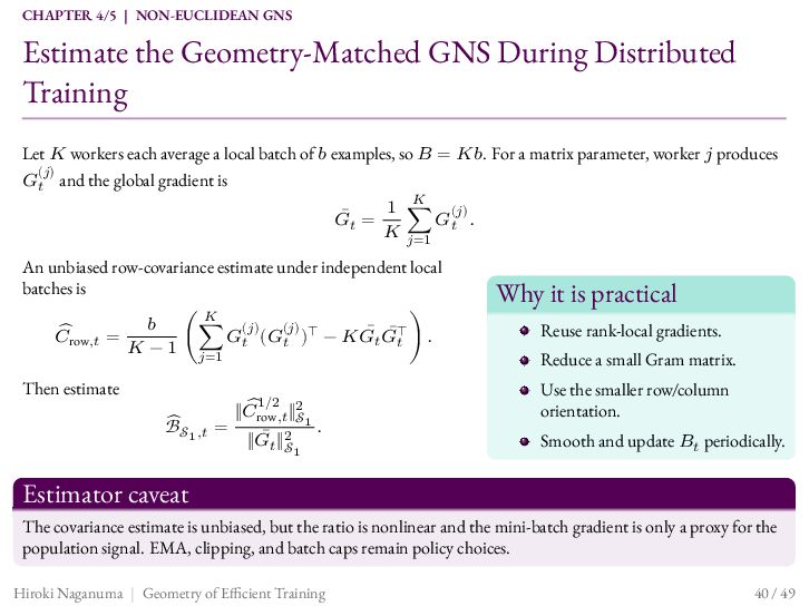
40. CHAPTER 4/5 | NON-EUCLIDEAN GNS Estimate the Geometry-Matched GNS During Distributed Training Let 𝐾 workers each average a local batch of 𝑏 examples, so 𝐵 = 𝐾𝑏. For a matrix parameter, worker 𝑗 produces (𝑗) 𝐺𝑡 and the global gradient is 𝐺𝑡̄ = 1 𝐾 (𝑗) ∑𝐺 . 𝐾 𝑗=1 𝑡 An unbiased row-covariance estimate under independent local batches is 𝐾 𝑏 (𝑗) (𝑗) ̂ ̄ (∑ 𝐺 (𝐺𝑡 )⊤ − 𝐾 𝐺𝑡̄ 𝐺⊤ 𝐶 row,𝑡 = 𝑡 ). 𝐾 − 1 𝑗=1 𝑡 Then estimate 1/2 ̂ ℬ 𝒮1 ,𝑡 = 2 ̂ ‖𝐶 row,𝑡 ‖𝒮1 . ‖𝐺𝑡̄ ‖2 𝒮1 Why it is practical Reuse rank-local gradients. Reduce a small Gram matrix. Use the smaller row/column orientation. Smooth and update 𝐵𝑡 periodically. Estimator caveat The covariance estimate is unbiased, but the ratio is nonlinear and the mini-batch gradient is only a proxy for the population signal. EMA, clipping, and batch caps remain policy choices. Hiroki Naganuma | Geometry of Efficient Training 40 / 49
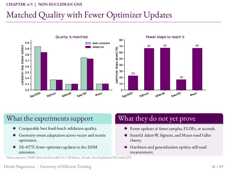
41. CHAPTER 4/5 | NON-EUCLIDEAN GNS Matched Quality with Fewer Optimizer Updates best constant adaptive GD SignS m Signu W Adam GD Spec Muon What the experiments support Fewer steps to reach it 80 optimizer steps saved (%) validation loss (lower better) Quality is matched 4.0 3.9 3.8 3.7 3.6 3.5 3.4 3.3 3.2 67 70 67 67 60 50 40 30 23 20 16 10 0 GD SignS m Signu W Adam GD Spec Muon What they do not yet prove Comparable best fixed-batch validation quality. Fewer updates ≠ fewer samples, FLOPs, or seconds. Geometry-aware adaptation across vector and matrix optimizers. Stateful AdamW, Signum, and Muon need fuller theory. 16–67% fewer optimizer updates in the 320M extension. Hardware and generalization optima still need measurement. Thesis extension: 320M Llama-family model, C4, 3.2B tokens, 10 seeds. Non-Euclidean GNS results [27]. Hiroki Naganuma | Geometry of Efficient Training 41 / 49
42. CHAPTER 5 OF 5 Decisions and Outlook From diagnosis to design
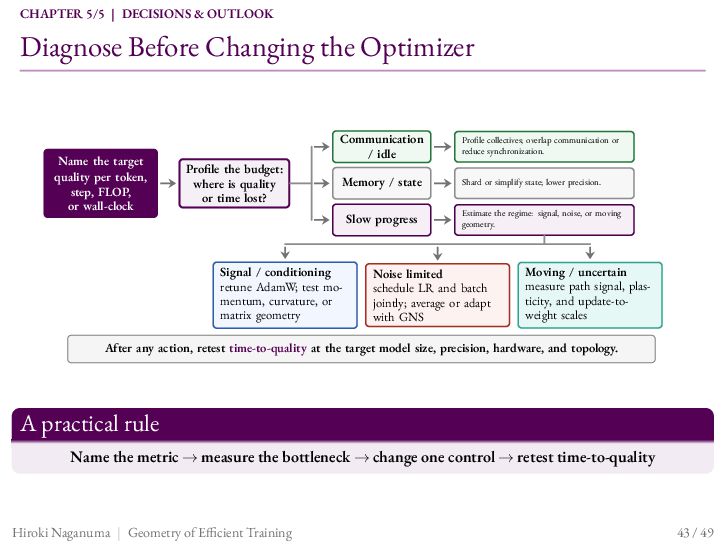
43. CHAPTER 5/5 | DECISIONS & OUTLOOK Diagnose Before Changing the Optimizer Name the target quality per token, step, FLOP, or wall-clock Profile the budget: where is quality or time lost? Communication / idle Profile collectives; overlap communication or reduce synchronization. Memory / state Shard or simplify state; lower precision. Slow progress Estimate the regime: signal, noise, or moving geometry. Signal / conditioning retune AdamW; test momentum, curvature, or matrix geometry Noise limited schedule LR and batch jointly; average or adapt with GNS Moving / uncertain measure path signal, plasticity, and update-toweight scales After any action, retest time-to-quality at the target model size, precision, hardware, and topology. A practical rule Name the metric → measure the bottleneck → change one control → retest time-to-quality Hiroki Naganuma | Geometry of Efficient Training 43 / 49
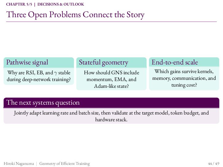
44. CHAPTER 5/5 | DECISIONS & OUTLOOK Three Open Problems Connect the Story Pathwise signal Stateful geometry Why are RSI, EB, and 𝛾 stable during deep-network training? How should GNS include momentum, EMA, and Adam-like state? End-to-end scale Which gains survive kernels, memory, communication, and tuning cost? The next systems question Jointly adapt learning rate and batch size, then validate at the target model, token budget, and hardware stack. Hiroki Naganuma | Geometry of Efficient Training 44 / 49
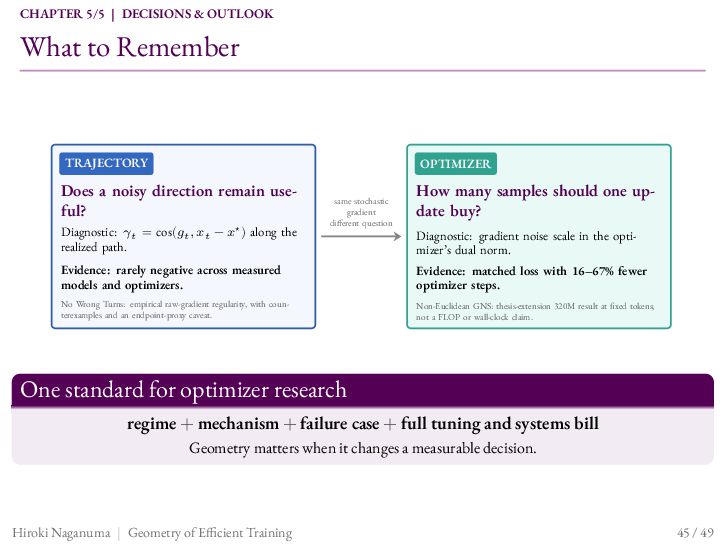
45. CHAPTER 5/5 | DECISIONS & OUTLOOK What to Remember TRAJECTORY OPTIMIZER Does a noisy direction remain useful? How many samples should one update buy? Diagnostic: 𝛾𝑡 = cos(𝑔𝑡 , 𝑥𝑡 − 𝑥 ) along the realized path. ⋆ same stochastic gradient different question Diagnostic: gradient noise scale in the optimizer’s dual norm. Evidence: rarely negative across measured models and optimizers. Evidence: matched loss with 16–67% fewer optimizer steps. No Wrong Turns: empirical raw-gradient regularity, with counterexamples and an endpoint-proxy caveat. Non-Euclidean GNS: thesis-extension 320M result at fixed tokens; not a FLOP or wall-clock claim. One standard for optimizer research regime + mechanism + failure case + full tuning and systems bill Geometry matters when it changes a measurable decision. Hiroki Naganuma | Geometry of Efficient Training 45 / 49
46. CHAPTER 5/5 | DECISIONS & OUTLOOK Acknowledgements: Advisors and Mentors PhD advisor I am deeply grateful to Ioannis Mitliagkas for his supervision, guidance, and support throughout my PhD. Research mentors Internship mentors Mila: Kilian Fatras and Kartik Ahuja. Early PhD support: Rio Yokota. Microsoft Research: Russell J. Hewett, Philipp A. Witte, Yin Tat Lee. Google DeepMind: George E. Dahl, Priya Kasimbeg, Sourabh Medapati, Shankar Krishnan, Atish Agarwala, Ran Tian. Meta: Hao-Jun Michael Shi, Parameswaran Raman. LinkedIn: Aman Gupta, Sathiya Keerthi Selvaraj, Haichao Wei, Mingzhou Zhou, Chengming Jiang. Professors and research guidance Irina Rish, Guillaume Rabusseau, Taiji Suzuki, Toyotaro Suzumura, Kota Ishikawa, Ikuro Sato, Atsushi Nitanda, Hideaki Iiduka, Hideyuki Kawashima, Akira Uehara, Takeru Sakurai, and Yoshiyuki Sankai. Hiroki Naganuma | Geometry of Efficient Training 46 / 49
47. CHAPTER 5/5 | DECISIONS & OUTLOOK Acknowledgements: Collaborators and Support Collaborators in this talk Broader thesis collaborations Charles Guille-Escuret, Kilian Fatras, Xinzhi Zhang, Man-Chung Yue, Philipp A. Witte, Russell J. Hewett, Yin Tat Lee, Shagun Gupta, Youssef Briki, Irina Rish, Parameswaran Raman, and Hao-Jun Michael Shi. Masanari Kimura (ZOZO, University of Melbourne), Ryotaro Shimizu (ZOZO, UC San Diego), Yuki Saito (ZOZO), Shiro Takagi, Ryuichiro Hataya, Seng Pei Liew, Junhyung Lyle Kim, Tetsuya Motokawa, Tatsuro Ide, Jumpei Nagase, and Masahiro Nomura. Research environment and support Thanks to Mila, Université de Montréal, and mentors and teams at Microsoft Research, Google DeepMind, Meta, and LinkedIn. This work was supported by Masason Foundation, RBC Borealis, JASSO, ANRI, Cyberdyne, Shigeta Education Foundation, NVIDIA, HPCI, JHPCN, ABCI, and TSUBAME. Hiroki Naganuma | Geometry of Efficient Training 47 / 49
48. CHAPTER 5/5 | DECISIONS & OUTLOOK Acknowledgements: Students I Mentored It was a privilege to mentor and collaborate with these talented students and early-career researchers during my PhD. Mentored students Mentored students (cont.) Youssef Briki (UdeM) Youssef Fadhloun (INSAT) Gaku Fujimori (Tokyo University of Science) Mahdi Ghaznavi (Mila) Laura Gomezjurado Gonzalez (Stanford University) Takafumi Horie (Kyoto University) Yoshikazu Ikeda (Osaka University) Haruka Kumagai (University of Tokyo) Kacem Mathlouthi (INSAT) Mark-Anthony Moisescu-Pareja (Mila) Sora Nakai (Kyoto University) Tatsuhiro Nakamori (Keio University) Yuji Naraki (Waseda University) Naoki Sato (Meiji University) Keigo Tada (Ritsumeikan University) Kaisei Takahashi (JAIST) Ganesh Talluri (BASIS Peoria) Mari Takeuchi (University College London) Ansh Tiwari (Caltech) Ryosuke Yamaki (Ritsumeikan University) Kotaro Yoshida (Science Tokyo) Hiroki Naganuma | Geometry of Efficient Training 48 / 49
49. Thank you. Questions and discussion
50. References I [1] J. Bernstein. Deriving muon, 2025. URL https://jeremybernste.in/writing/deriving- muon. [2] J. Bernstein and L. Newhouse. Old optimizer, new norm: An anthology. arXiv preprint arXiv:2409.20325, 2024. [3] J. Bernstein, Y.-X. Wang, K. Azizzadenesheli, and A. Anandkumar. signsgd: Compressed optimisation for non-convex problems. In International Conference on Machine Learning, pages 560–569. PMLR, 2018. [4] L. Bottou, F. E. Curtis, and J. Nocedal. Optimization methods for large-scale machine learning. SIAM Review, 60(2):223–311, 2018. doi: 10.1137/16M1080173. [5] D. Choi, C. J. Shallue, Z. Nado, J. Lee, C. J. Maddison, and G. E. Dahl. On empirical comparisons of optimizers for deep learning. arXiv preprint arXiv:1910.05446, 2019. URL https://arxiv.org/abs/1910.05446. [6] Essential AI, I. Shah, A. M. Polloreno, K. Stratos, P. Monk, A. Chaluvaraju, A. Hojel, A. Ma, et al. Practical efficiency of muon for pretraining. arXiv preprint arXiv:2505.02222, 2025. URL https://arxiv.org/abs/2505.02222. [7] C. Guille-Escuret, H. Naganuma, K. Fatras, and I. Mitliagkas. No wrong turns: The simple geometry of neural networks optimization paths. In International Conference on Machine Learning (ICML), 2024. [8] V. Gupta, T. Koren, and Y. Singer. Shampoo: Preconditioned stochastic tensor optimization. In International Conference on Machine Learning, 2018. [9] E. Hoffer, I. Hubara, and D. Soudry. Train longer, generalize better: closing the generalization gap in large batch training of neural networks. Advances in neural information processing systems, 30, 2017. [10] J. Hoffmann, S. Borgeaud, A. Mensch, E. Buchatskaya, T. Cai, E. Rutherford, D. d. L. Casas, L. A. Hendricks, J. Welbl, A. Clark, et al. Training compute-optimal large language models. arXiv preprint arXiv:2203.15556, 2022. [11] K. Jordan, Y. Jin, V. Boza, Y. Jiacheng, F. Cesista, L. Newhouse, and J. Bernstein. Muon: An optimizer for hidden layers in neural networks. https://kellerjordan.github.io/posts/muon/, 2024. Accessed: 2025-7-3. [12] J. Kaplan, S. McCandlish, T. Henighan, T. B. Brown, B. Chess, R. Child, S. Gray, A. Radford, J. Wu, and D. Amodei. Scaling laws for neural language models. arXiv preprint arXiv:2001.08361, 2020. [13] S. P. Karimireddy, Q. Rebjock, S. Stich, and M. Jaggi. Error feedback fixes SignSGD and other gradient compression schemes. In International Conference on Machine Learning, 2019. [14] P. Kasimbeg, F. Schneider, R. Eschenhagen, J. Bae, C. S. Sastry, M. Saroufim, B. Feng, L. Wright, E. Z. Yang, Z. Nado, S. Medapati, P. Hennig, M. Rabbat, and G. E. Dahl. Accelerating neural network training: An analysis of the AlgoPerf competition. In International Conference on Learning Representations, 2025. URL https://openreview.net/forum?id=CtM5xjRSfm. [15] N. S. Keskar, D. Mudigere, J. Nocedal, M. Smelyanskiy, and P. T. P. Tang. On large-batch training for deep learning: Generalization gap and sharp minima. arXiv preprint arXiv:1609.04836, 2016. [16] D. P. Kingma and J. Ba. Adam: A method for stochastic optimization. arXiv preprint arXiv:1412.6980, 2014.
51. References II [17] A. Koloskova, N. Loizou, S. Boreiri, M. Jaggi, and S. Stich. A unified theory of decentralized SGD with changing topology and local updates. International Conference on Machine Learning, 2020. [18] J. Liu, J. Su, X. Yao, Z. Jiang, G. Lai, Y. Du, Y. Qin, W. Xu, E. Lu, J. Yan, et al. Muon is scalable for LLM training. arXiv preprint arXiv:2502.16982, 2025. [19] I. Loshchilov and F. Hutter. Decoupled weight decay regularization. arXiv preprint arXiv:1711.05101, 2017. [20] J. Martens. Deep learning via hessian-free optimization. In Proceedings of the 27th International Conference on Machine Learning, pages 735–742, 2010. URL https://icml.cc/2010/papers/458.pdf. [21] J. Martens and R. Grosse. Optimizing neural networks with kronecker-factored approximate curvature. In Proceedings of the 32nd International Conference on Machine Learning, volume 37 of Proceedings of Machine Learning Research, pages 2408–2417, 2015. URL https://proceedings.mlr.press/v37/martens15.html. [22] D. Masters and C. Luschi. Revisiting small batch training for deep neural networks. arXiv preprint arXiv:1804.07612, 2018. [23] S. McCandlish, J. Kaplan, D. Amodei, and O. D. Team. An empirical model of large-batch training. arXiv preprint arXiv:1812.06162, 2018. [24] MLCommons. MLCommons announces results for the first AlgoPerf training algorithms competition. https://mlcommons.org/2024/08/mlc-algoperf- benchmark- competition/, 2024. [25] Z. Nado, J. M. Gilmer, C. J. Shallue, R. Anil, and G. E. Dahl. A large batch optimizer reality check: Traditional, generic optimizers suffice across batch sizes. arXiv preprint arXiv:2102.06356, 2021. [26] H. Naganuma, L. Gomezjurado Gonzalez, M. Ghaznavi, and I. Mitliagkas. The geometry of spectral gradient descent: Layerwise criteria for SignSGD vs SpecSGD. In ICLR 2026 Workshop on Geometry-grounded Representation Learning and Generative Modeling, 2026. [27] H. Naganuma, S. Gupta, Y. Briki, I. Mitliagkas, I. Rish, P. Raman, and H.-J. M. Shi. Adaptive batch sizes using non-euclidean gradient noise scales for stochastic sign and spectral descent. International Conference on Machine Learning (ICML), 2026. [28] Y. Nesterov. Introductory Lectures on Convex Optimization: A Basic Course, volume 87 of Applied Optimization. Kluwer Academic Publishers, 2004. [29] R. M. Schmidt, F. Schneider, and P. Hennig. Descending through a crowded valley: Benchmarking deep learning optimizers. In Proceedings of the 38th International Conference on Machine Learning, volume 139 of Proceedings of Machine Learning Research, pages 9367–9376, 2021. URL https://proceedings.mlr.press/v139/schmidt21a.html. [30] C. J. Shallue, J. Lee, J. Antognini, J. Sohl-Dickstein, R. Frostig, and G. E. Dahl. Measuring the effects of data parallelism on neural network training. Journal of Machine Learning Research, 20(112):1–49, 2019. [31] H.-J. M. Shi, T.-H. Lee, S. Iwasaki, J. Gallego-Posada, Z. Li, K. Rangadurai, D. Mudigere, and M. Rabbat. A distributed data-parallel PyTorch implementation of the distributed Shampoo optimizer for training neural networks at-scale. arXiv preprint arXiv:2309.06497, 2023. URL https://arxiv.org/abs/2309.06497. [32] S. L. Smith, P.-J. Kindermans, C. Ying, and Q. V. Le. Don’t decay the learning rate, increase the batch size. arXiv preprint arXiv:1711.00489, 2017. [33] H. Zhang, D. Morwani, N. Vyas, J. Wu, D. Zou, U. Ghai, D. Foster, and S. Kakade. How does critical batch size scale in pre-training? arXiv preprint arXiv:2410.21676, 2024.
52. Appendix: Map of Backup Material A Background / prerequisites B Gradient signal: pathwise measurements and Q&A C Optimizer geometry: Non-Euclidean GNS theory, implementation, results, and Q&A D General questions about the two featured works Hiroki Naganuma | Geometry of Efficient Training A-1 / 64
53. Appendix A: Background / Prerequisites SGD, loss landscapes, and optimizer geometry. Hiroki Naganuma | Geometry of Efficient Training A-2 / 64
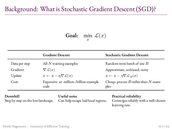
54. Background: What is Stochastic Gradient Descent (SGD)? Goal: min ℒ(𝑥) 𝑥 Gradient Descent Stochastic Gradient Descent Data per step All 𝑁 training examples Random mini-batch of size 𝐵 Gradient ∇ℒ(𝑥) Approximate, unbiased, noisy Update 𝑥 ← 𝑥 − 𝜂∇ℒ(𝑥) 𝑥 ← 𝑥 − 𝜂∇ℒℬ (𝑥) Cost Expensive at million-/billion-example scale Cheap: process 𝐵 rather than 𝑁 examples Downhill Step by step on the loss landscape. Useful noise Can help escape bad local regions. Hiroki Naganuma | Geometry of Efficient Training Practical reliability Converges reliably with a well-chosen learning rate. A-3 / 64
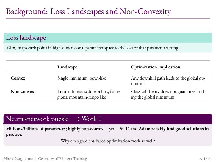
55. Background: Loss Landscapes and Non-Convexity Loss landscape ℒ(𝑥) maps each point in high-dimensional parameter space to the loss of that parameter setting. Landscape Optimization implication Convex Single minimum; bowl-like Any downhill path leads to the global optimum Non-convex Local minima, saddle points, flat regions; mountain-range-like Classical theory does not guarantee finding the global minimum Neural-network puzzle ⟶ Work 1 Millions/billions of parameters; highly non-convex yet SGD and Adam reliably find good solutions in practice. Why does gradient-based optimization work so well? Hiroki Naganuma | Geometry of Efficient Training A-4 / 64
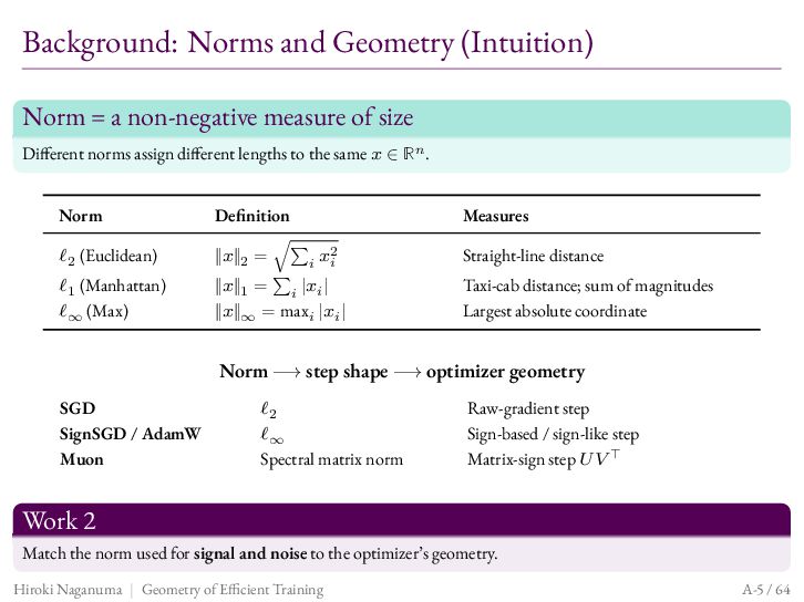
56. Background: Norms and Geometry (Intuition) Norm = a non-negative measure of size Different norms assign different lengths to the same 𝑥 ∈ ℝ𝑛 . Norm Definition Measures ℓ2 (Euclidean) ‖𝑥‖2 = √∑𝑖 𝑥2𝑖 Straight-line distance ℓ1 (Manhattan) ℓ∞ (Max) ‖𝑥‖1 = ∑𝑖 |𝑥𝑖 | ‖𝑥‖∞ = max𝑖 |𝑥𝑖 | Taxi-cab distance; sum of magnitudes Largest absolute coordinate Norm ⟶ step shape ⟶ optimizer geometry SGD SignSGD / AdamW Muon ℓ2 ℓ∞ Spectral matrix norm Raw-gradient step Sign-based / sign-like step Matrix-sign step 𝑈𝑉 ⊤ Work 2 Match the norm used for signal and noise to the optimizer’s geometry. Hiroki Naganuma | Geometry of Efficient Training A-5 / 64
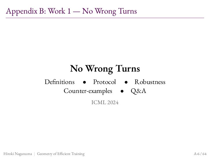
57. Appendix B: Work 1 — No Wrong Turns No Wrong Turns Definitions • Protocol • Robustness Counter-examples • Q&A ICML 2024 Hiroki Naganuma | Geometry of Efficient Training A-6 / 64
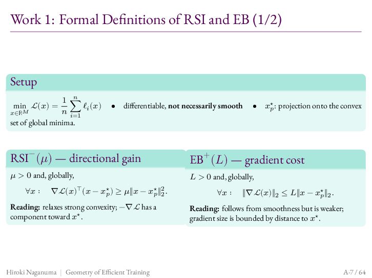
58. Work 1: Formal Definitions of RSI and EB (1/2) Setup 1 𝑛 ∑ ℓ (𝑥) 𝑛 𝑖=1 𝑖 set of global minima. min ℒ(𝑥) = 𝑥∈ℝ𝑀 • differentiable, not necessarily smooth • 𝑥⋆𝑝 : projection onto the convex RSI− (𝜇) — directional gain EB+ (𝐿) — gradient cost 𝜇 > 0 and, globally, 𝐿 > 0 and, globally, ∀𝑥 ∶ ∇ℒ(𝑥)⊤ (𝑥 − 𝑥⋆𝑝 ) ≥ 𝜇‖𝑥 − 𝑥⋆𝑝 ‖22 . Reading: relaxes strong convexity; −∇ℒ has a component toward 𝑥⋆ . Hiroki Naganuma | Geometry of Efficient Training ∀𝑥 ∶ ‖∇ℒ(𝑥)‖2 ≤ 𝐿‖𝑥 − 𝑥⋆𝑝 ‖2 . Reading: follows from smoothness but is weaker; gradient size is bounded by distance to 𝑥⋆ . A-7 / 64
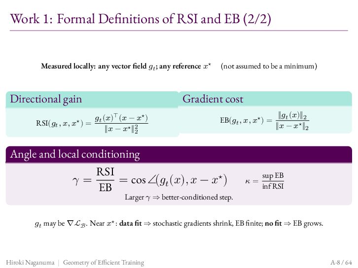
59. Work 1: Formal Definitions of RSI and EB (2/2) Measured locally: any vector field 𝑔𝑡 ; any reference 𝑥⋆ (not assumed to be a minimum) Gradient cost Directional gain 𝑔 (𝑥)⊤ (𝑥 − 𝑥⋆ ) RSI(𝑔𝑡 , 𝑥, 𝑥⋆ ) = 𝑡 ‖𝑥 − 𝑥⋆ ‖22 EB(𝑔𝑡 , 𝑥, 𝑥⋆ ) = Angle and local conditioning RSI 𝛾= = cos ∠(𝑔𝑡 (𝑥), 𝑥 − 𝑥⋆ ) EB 𝜅= ‖𝑔𝑡 (𝑥)‖2 ‖𝑥 − 𝑥⋆ ‖2 sup EB inf RSI Larger 𝛾 ⇒ better-conditioned step. 𝑔𝑡 may be ∇ℒℬ . Near 𝑥⋆ : data fit ⇒ stochastic gradients shrink, EB finite; no fit ⇒ EB grows. Hiroki Naganuma | Geometry of Efficient Training A-8 / 64
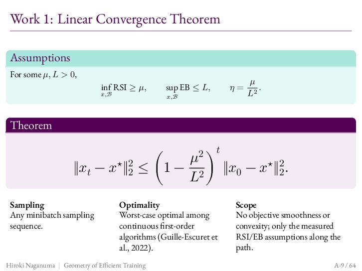
60. Work 1: Linear Convergence Theorem Assumptions For some 𝜇, 𝐿 > 0, inf RSI ≥ 𝜇, 𝑥,ℬ sup EB ≤ 𝐿, 𝑥,ℬ 𝜂= 𝜇 . 𝐿2 Theorem 𝑡 𝜇2 ⋆ 2 ‖𝑥𝑡 − 𝑥 ‖2 ≤ (1 − 2 ) ‖𝑥0 − 𝑥⋆ ‖22 . 𝐿 Sampling Any minibatch sampling sequence. Optimality Worst-case optimal among continuous first-order algorithms (Guille-Escuret et al., 2022). Hiroki Naganuma | Geometry of Efficient Training Scope No objective smoothness or convexity; only the measured RSI/EB assumptions along the path. A-9 / 64
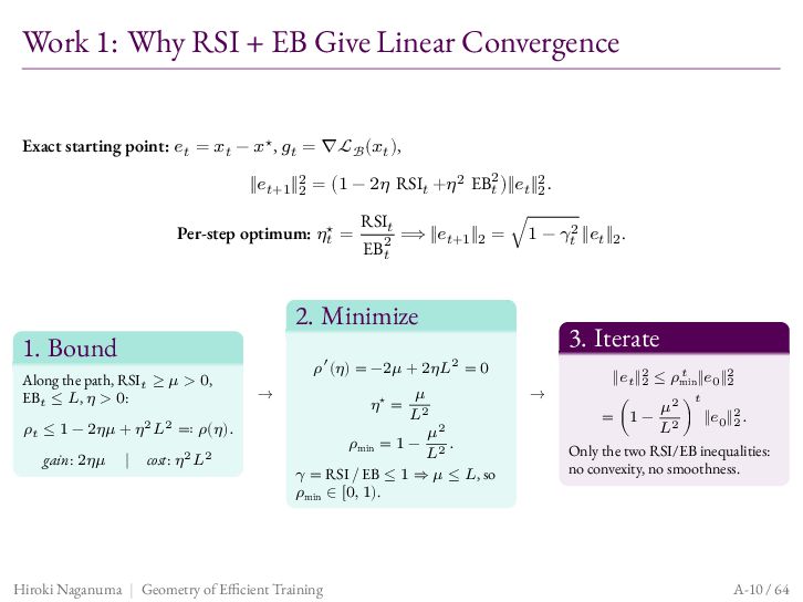
61. Work 1: Why RSI + EB Give Linear Convergence Exact starting point: 𝑒𝑡 = 𝑥𝑡 − 𝑥⋆ , 𝑔𝑡 = ∇ℒℬ (𝑥𝑡 ), ‖𝑒𝑡+1 ‖22 = (1 − 2𝜂 RSI𝑡 +𝜂2 EB2𝑡 )‖𝑒𝑡 ‖22 . Per-step optimum: 𝜂𝑡⋆ = EB2𝑡 ⟹ ‖𝑒𝑡+1 ‖2 = √1 − 𝛾𝑡2 ‖𝑒𝑡 ‖2 . 2. Minimize 1. Bound Along the path, RSI𝑡 ≥ 𝜇 > 0, EB𝑡 ≤ 𝐿, 𝜂 > 0: 2 2 𝜌𝑡 ≤ 1 − 2𝜂𝜇 + 𝜂 𝐿 =∶ 𝜌(𝜂). gain: 2𝜂𝜇 RSI𝑡 | cost: 𝜂2 𝐿2 3. Iterate 𝜌′ (𝜂) = −2𝜇 + 2𝜂𝐿2 = 0 → 𝜇 𝜂 = 2 𝐿 𝜇2 𝜌min = 1 − 2 . 𝐿 𝛾 = RSI / EB ≤ 1 ⇒ 𝜇 ≤ 𝐿, so 𝜌min ∈ [0, 1). Hiroki Naganuma | Geometry of Efficient Training ⋆ → 𝑡 ‖𝑒𝑡 ‖22 ≤ 𝜌min ‖𝑒0 ‖22 𝑡 = (1 − 𝜇2 ) ‖𝑒0 ‖22 . 𝐿2 Only the two RSI/EB inequalities: no convexity, no smoothness. A-10 / 64
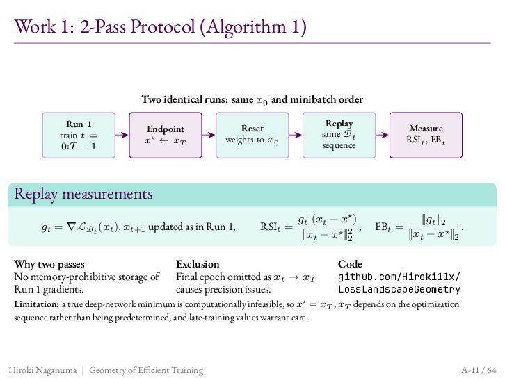
62. Work 1: 2-Pass Protocol (Algorithm 1) Two identical runs: same 𝑥0 and minibatch order Run 1 train 𝑡 = 0∶𝑇 − 1 Endpoint 𝑥⋆ ← 𝑥𝑇 Replay same ℬ𝑡 sequence Reset weights to 𝑥0 Measure RSI𝑡 , EB𝑡 Replay measurements 𝑔𝑡 = ∇ℒℬ𝑡 (𝑥𝑡 ), 𝑥𝑡+1 updated as in Run 1, Why two passes No memory-prohibitive storage of Run 1 gradients. RSI𝑡 = 𝑔𝑡⊤ (𝑥𝑡 − 𝑥⋆ ) , ‖𝑥𝑡 − 𝑥⋆ ‖22 Exclusion Final epoch omitted as 𝑥𝑡 → 𝑥𝑇 causes precision issues. EB𝑡 = ‖𝑔𝑡 ‖2 . ‖𝑥𝑡 − 𝑥⋆ ‖2 Code github.com/Hiroki11x/ LossLandscapeGeometry Limitation: a true deep-network minimum is computationally infeasible, so 𝑥⋆ = 𝑥𝑇 ; 𝑥𝑇 depends on the optimization sequence rather than being predetermined, and late-training values warrant care. Hiroki Naganuma | Geometry of Efficient Training A-11 / 64
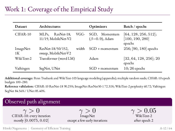
63. Work 1: Coverage of the Empirical Study Dataset Architectures Optimizers Batch / epochs CIFAR-10 MLPs, ResNet-18, 11/19, MobileNet-V2 VGG- SGD, Momentum (𝛽=0.9), Adam ImageNet1K WikiText-2 ResNet-18/50/152, width sweep, MobileNet-V2 Transformer (word LM) SGD + momentum [64, 128, 256, 512]; [100, 190, 280] epochs 256; [90, 180] epochs Adam Vaihingen SegNet, UNet SGD + momentum [32, 64, 128, 256]; 20 epochs 10; 26 epochs Additional coverage: Penn Treebank and WikiText-103 language modeling (appendix); multiple random seeds; CIFAR-10 epoch budgets 100–280. Reference validation: CIFAR-10 ResNet-18 90.25%; ImageNet ResNet50-1 72.31%; WikiText-2 perplexity 60.72; Vaihingen SegNet 84.56% / UNet 85.40%. Observed path alignment 𝛾>0 CIFAR-10: every iteration mostly [0.0075, 0.02] 𝛾>0 ImageNet except a few early iterations Hiroki Naganuma | Geometry of Efficient Training 𝛾 > 0.05 WikiText-2 after epoch 2 A-12 / 64
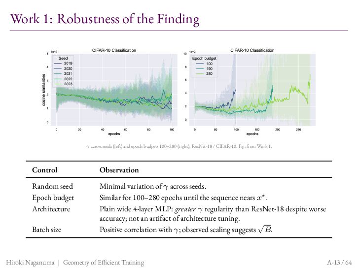
64. Work 1: Robustness of the Finding 5 1e 2 CIFAR-10 Classification cosine similarities Epoch budget 2019 2020 2021 2022 2023 4 3 CIFAR-10 Classification 10 1e 2 Seed 100 190 280 8 6 2 4 1 2 0 0 0 20 40 epochs 60 80 100 0 50 100 150 epochs 200 250 𝛾 across seeds (left) and epoch budgets 100–280 (right), ResNet-18 / CIFAR-10. Fig. from Work 1. Control Observation Random seed Epoch budget Architecture Minimal variation of 𝛾 across seeds. Similar for 100–280 epochs until the sequence nears 𝑥⋆ . Plain wide 4-layer MLP: greater 𝛾 regularity than ResNet-18 despite worse accuracy; not an artifact of architecture tuning. √ Positive correlation with 𝛾; observed scaling suggests 𝐵. Batch size Hiroki Naganuma | Geometry of Efficient Training A-13 / 64
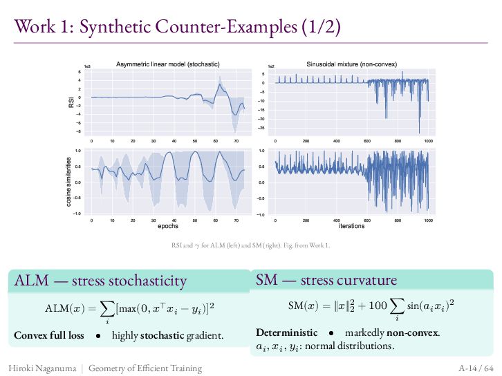
65. Work 1: Synthetic Counter-Examples (1/2) 6 Asymmetric linear model (stochastic) 1e3 0 RSI 2 5 0 10 2 15 4 20 6 25 8 0 cosine similarities Sinusoidal mixture (non-convex) 1e2 5 4 10 20 30 40 50 60 70 1.0 1.0 0.5 0.5 0.0 0.0 0.5 0.5 1.0 0 10 20 30 40 epochs 50 60 70 1.0 0 200 400 600 800 1000 0 200 400 600 800 1000 iterations RSI and 𝛾 for ALM (left) and SM (right). Fig. from Work 1. ALM — stress stochasticity ALM(𝑥) = ∑[max(0, 𝑥⊤ 𝑥𝑖 − 𝑦𝑖 )]2 𝑖 Convex full loss • highly stochastic gradient. Hiroki Naganuma | Geometry of Efficient Training SM — stress curvature SM(𝑥) = ‖𝑥‖22 + 100 ∑ sin(𝑎𝑖 𝑥𝑖 )2 𝑖 Deterministic • markedly non-convex. 𝑎𝑖 , 𝑥𝑖 , 𝑦𝑖 : normal distributions. A-14 / 64
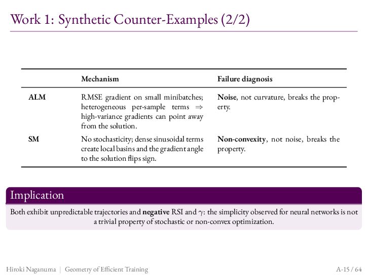
66. Work 1: Synthetic Counter-Examples (2/2) Mechanism Failure diagnosis ALM RMSE gradient on small minibatches; heterogeneous per-sample terms ⇒ high-variance gradients can point away from the solution. Noise, not curvature, breaks the property. SM No stochasticity; dense sinusoidal terms create local basins and the gradient angle to the solution flips sign. Non-convexity, not noise, breaks the property. Implication Both exhibit unpredictable trajectories and negative RSI and 𝛾: the simplicity observed for neural networks is not a trivial property of stochastic or non-convex optimization. Hiroki Naganuma | Geometry of Efficient Training A-15 / 64
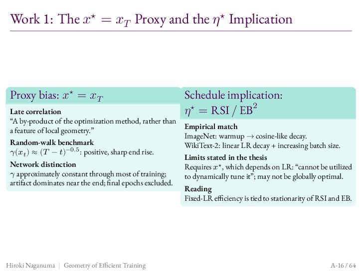
67. Work 1: The 𝑥⋆ = 𝑥𝑇 Proxy and the 𝜂⋆ Implication Proxy bias: 𝑥⋆ = 𝑥𝑇 Late correlation “A by-product of the optimization method, rather than a feature of local geometry.” Random-walk benchmark 𝛾(𝑥𝑡 ) ≈ (𝑇 − 𝑡)−0.5 : positive, sharp end rise. Network distinction 𝛾 approximately constant through most of training; artifact dominates near the end; final epochs excluded. Hiroki Naganuma | Geometry of Efficient Training Schedule implication: 𝜂⋆ = RSI / EB2 Empirical match ImageNet: warmup → cosine-like decay. WikiText-2: linear LR decay + increasing batch size. Limits stated in the thesis Requires 𝑥⋆ , which depends on LR: “cannot be utilized to dynamically tune it”; may not be globally optimal. Reading Fixed-LR efficiency is tied to stationarity of RSI and EB. A-16 / 64
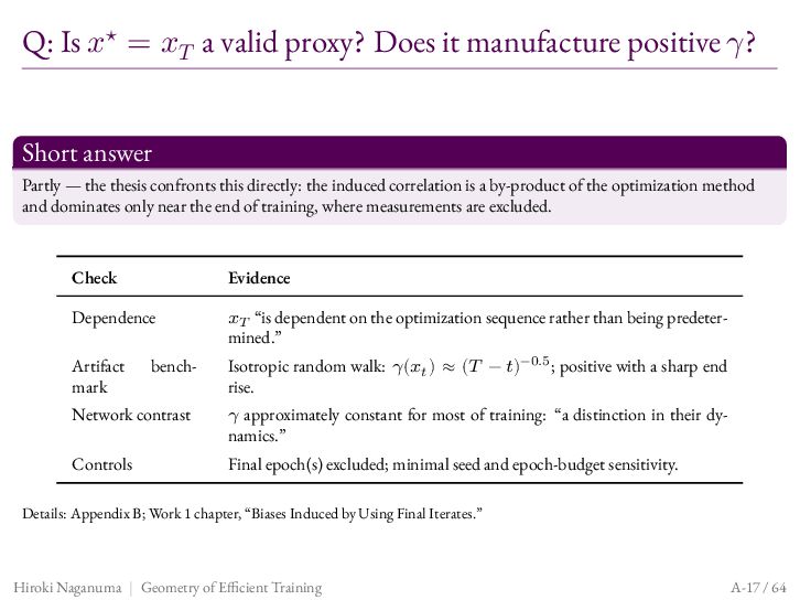
68. Q: Is 𝑥⋆ = 𝑥𝑇 a valid proxy? Does it manufacture positive 𝛾? Short answer Partly — the thesis confronts this directly: the induced correlation is a by-product of the optimization method and dominates only near the end of training, where measurements are excluded. Check Evidence Dependence 𝑥𝑇 “is dependent on the optimization sequence rather than being predetermined.” Artifact mark bench- Isotropic random walk: 𝛾(𝑥𝑡 ) ≈ (𝑇 − 𝑡)−0.5 ; positive with a sharp end rise. Network contrast 𝛾 approximately constant for most of training: “a distinction in their dynamics.” Controls Final epoch(s) excluded; minimal seed and epoch-budget sensitivity. Details: Appendix B; Work 1 chapter, “Biases Induced by Using Final Iterates.” Hiroki Naganuma | Geometry of Efficient Training A-17 / 64
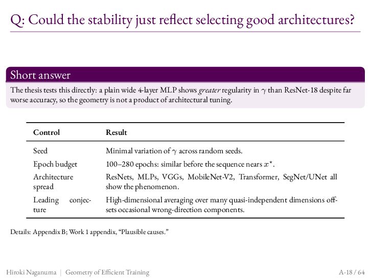
69. Q: Could the stability just reflect selecting good architectures? Short answer The thesis tests this directly: a plain wide 4-layer MLP shows greater regularity in 𝛾 than ResNet-18 despite far worse accuracy, so the geometry is not a product of architectural tuning. Control Result Seed Minimal variation of 𝛾 across random seeds. Epoch budget 100–280 epochs: similar before the sequence nears 𝑥⋆ . Architecture spread ResNets, MLPs, VGGs, MobileNet-V2, Transformer, SegNet/UNet all show the phenomenon. Leading ture High-dimensional averaging over many quasi-independent dimensions offsets occasional wrong-direction components. conjec- Details: Appendix B; Work 1 appendix, “Plausible causes.” Hiroki Naganuma | Geometry of Efficient Training A-18 / 64
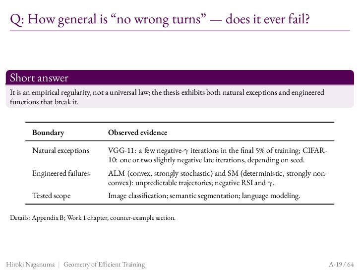
70. Q: How general is “no wrong turns” — does it ever fail? Short answer It is an empirical regularity, not a universal law; the thesis exhibits both natural exceptions and engineered functions that break it. Boundary Observed evidence Natural exceptions VGG-11: a few negative-𝛾 iterations in the final 5% of training; CIFAR10: one or two slightly negative late iterations, depending on seed. Engineered failures ALM (convex, strongly stochastic) and SM (deterministic, strongly nonconvex): unpredictable trajectories; negative RSI and 𝛾. Tested scope Image classification; semantic segmentation; language modeling. Details: Appendix B; Work 1 chapter, counter-example section. Hiroki Naganuma | Geometry of Efficient Training A-19 / 64
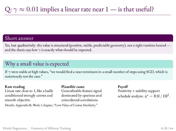
71. Q: 𝛾 ≈ 0.01 implies a linear rate near 1 — is that useful? Short answer Yes, but qualitatively: the value is structural (positive, stable, predictable geometry), not a tight runtime bound — and the thesis says low 𝛾 is exactly what should be expected. Why a small value is expected If 𝛾 were stable at high values, “we would find a near-minimum in a small number of steps using SGD, which is notoriously not the case.” Rate reading Linear rate close to 1, like a badly conditioned strongly convex and smooth objective. Plausible cause Generalizable-feature signal dominated by spurious and coincidental correlations. Payoff Positivity + stability support schedule analysis: 𝜂⋆ = RSI / EB2 . Details: Appendix B; Work 1 chapter, “Low Value of Cosine Similarity.” Hiroki Naganuma | Geometry of Efficient Training A-20 / 64
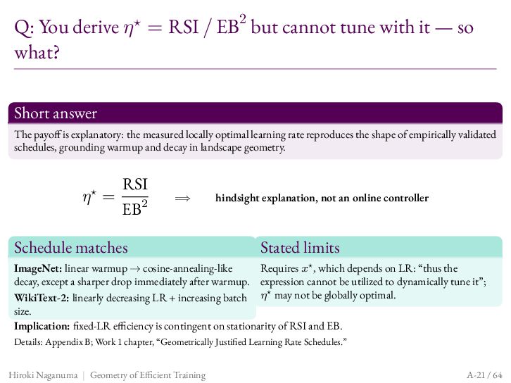
72. Q: You derive 𝜂⋆ = RSI / EB2 but cannot tune with it — so what? Short answer The payoff is explanatory: the measured locally optimal learning rate reproduces the shape of empirically validated schedules, grounding warmup and decay in landscape geometry. 𝜂⋆ = RSI EB2 ⟹ Schedule matches hindsight explanation, not an online controller Stated limits ImageNet: linear warmup → cosine-annealing-like Requires 𝑥⋆ , which depends on LR: “thus the decay, except a sharper drop immediately after warmup. expression cannot be utilized to dynamically tune it”; ⋆ WikiText-2: linearly decreasing LR + increasing batch 𝜂 may not be globally optimal. size. Implication: fixed-LR efficiency is contingent on stationarity of RSI and EB. Details: Appendix B; Work 1 chapter, “Geometrically Justified Learning Rate Schedules.” Hiroki Naganuma | Geometry of Efficient Training A-21 / 64
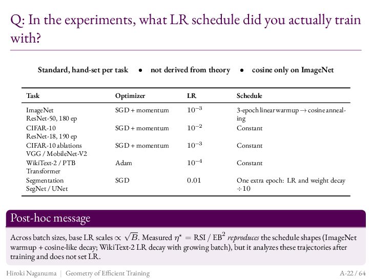
73. Q: In the experiments, what LR schedule did you actually train with? Standard, hand-set per task • not derived from theory LR • cosine only on ImageNet Task Optimizer ImageNet ResNet-50, 180 ep CIFAR-10 ResNet-18, 190 ep CIFAR-10 ablations VGG / MobileNet-V2 WikiText-2 / PTB Transformer Segmentation SegNet / UNet SGD + momentum 10 SGD + momentum 10−2 3-epoch linear warmup → cosine annealing Constant SGD + momentum 10−3 Constant −4 −3 Schedule Adam 10 Constant SGD 0.01 One extra epoch: LR and weight decay ÷10 Post-hoc message √ Across batch sizes, base LR scales ∝ 𝐵. Measured 𝜂⋆ = RSI / EB2 reproduces the schedule shapes (ImageNet warmup + cosine-like decay; WikiText-2 LR decay with growing batch), but it analyzes these trajectories after training and does not set LR. Hiroki Naganuma | Geometry of Efficient Training A-22 / 64
74. Appendix C: Work 2 — Non-Euclidean GNS Non-Euclidean GNS Theory • Norms • Implementation Results • Q&A ICML 2026 Hiroki Naganuma | Geometry of Efficient Training A-23 / 64
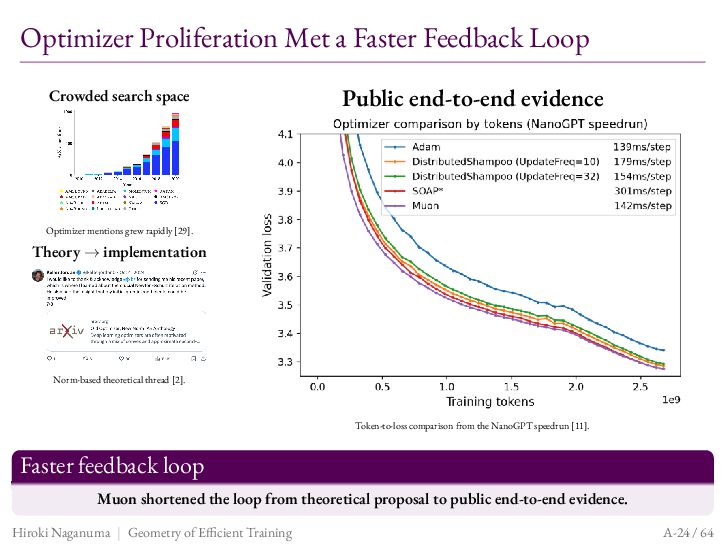
75. Optimizer Proliferation Met a Faster Feedback Loop Crowded search space Public end-to-end evidence Optimizer mentions grew rapidly [29]. Theory → implementation Norm-based theoretical thread [2]. Token-to-loss comparison from the NanoGPT speedrun [11]. Faster feedback loop Muon shortened the loop from theoretical proposal to public end-to-end evidence. Hiroki Naganuma | Geometry of Efficient Training A-24 / 64
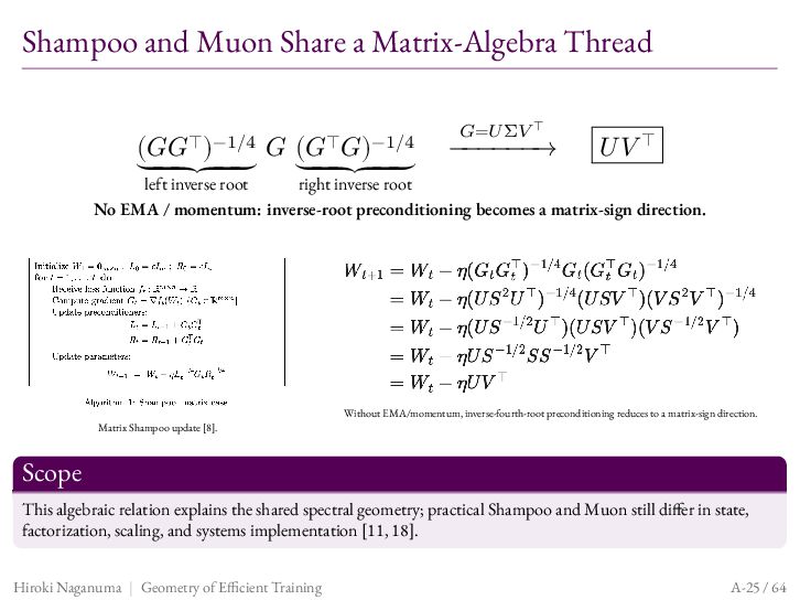
76. Shampoo and Muon Share a Matrix-Algebra Thread ⊤ )−1/4 𝐺 (𝐺⊤ 𝐺)−1/4 (𝐺𝐺 ⏟ ⏟⏟ ⏟⏟ ⏟⏟⏟⏟⏟ 𝐺=𝑈Σ𝑉 ⊤ −−−−−−→ 𝑈𝑉 ⊤ right inverse root left inverse root No EMA / momentum: inverse-root preconditioning becomes a matrix-sign direction. Without EMA/momentum, inverse-fourth-root preconditioning reduces to a matrix-sign direction. Matrix Shampoo update [8]. Scope This algebraic relation explains the shared spectral geometry; practical Shampoo and Muon still differ in state, factorization, scaling, and systems implementation [11, 18]. Hiroki Naganuma | Geometry of Efficient Training A-25 / 64
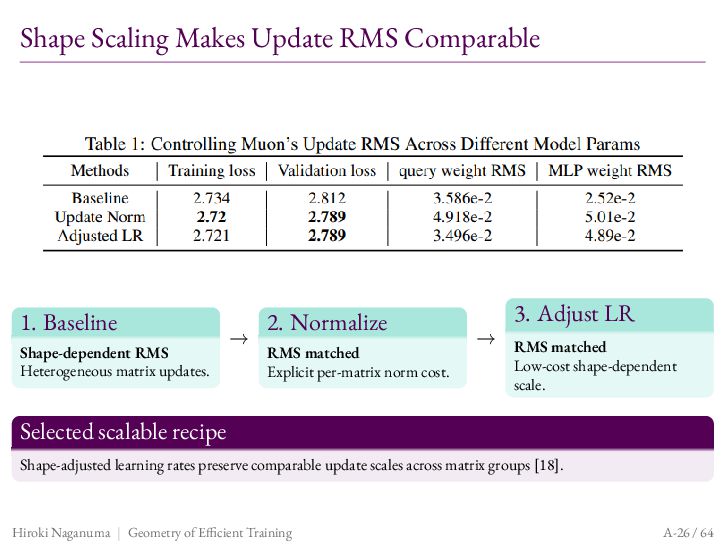
77. Shape Scaling Makes Update RMS Comparable 1. Baseline Shape-dependent RMS Heterogeneous matrix updates. → 2. Normalize RMS matched Explicit per-matrix norm cost. 3. Adjust LR → RMS matched Low-cost shape-dependent scale. Selected scalable recipe Shape-adjusted learning rates preserve comparable update scales across matrix groups [18]. Hiroki Naganuma | Geometry of Efficient Training A-26 / 64
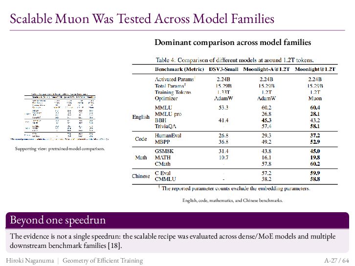
78. Scalable Muon Was Tested Across Model Families Dominant comparison across model families Supporting view: pretrained-model comparison. English, code, mathematics, and Chinese benchmarks. Beyond one speedrun The evidence is not a single speedrun: the scalable recipe was evaluated across dense/MoE models and multiple downstream benchmark families [18]. Hiroki Naganuma | Geometry of Efficient Training A-27 / 64
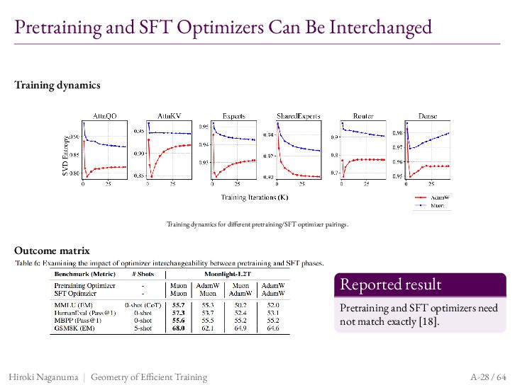
79. Pretraining and SFT Optimizers Can Be Interchanged Training dynamics Training dynamics for different pretraining/SFT optimizer pairings. Outcome matrix Reported result Pretraining and SFT optimizers need not match exactly [18]. Hiroki Naganuma | Geometry of Efficient Training A-28 / 64
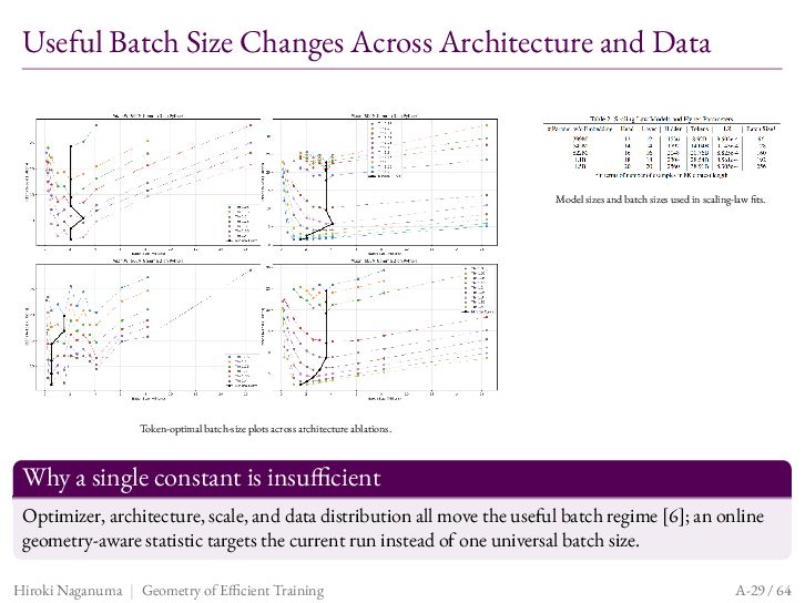
80. Useful Batch Size Changes Across Architecture and Data Model sizes and batch sizes used in scaling-law fits. Token-optimal batch-size plots across architecture ablations. Why a single constant is insufficient Optimizer, architecture, scale, and data distribution all move the useful batch regime [6]; an online geometry-aware statistic targets the current run instead of one universal batch size. Hiroki Naganuma | Geometry of Efficient Training A-29 / 64
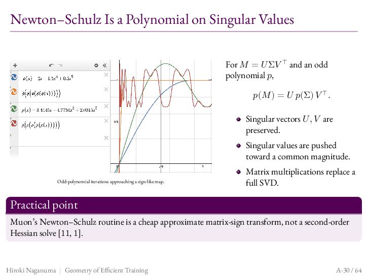
81. Newton–Schulz Is a Polynomial on Singular Values For 𝑀 = 𝑈 Σ𝑉 ⊤ and an odd polynomial 𝑝, 𝑝(𝑀 ) = 𝑈 𝑝(Σ) 𝑉 ⊤ . Singular vectors 𝑈 , 𝑉 are preserved. Singular values are pushed toward a common magnitude. Odd-polynomial iterations approaching a sign-like map. Matrix multiplications replace a full SVD. Practical point Muon’s Newton–Schulz routine is a cheap approximate matrix-sign transform, not a second-order Hessian solve [11, 1]. Hiroki Naganuma | Geometry of Efficient Training A-30 / 64
82. Classical Gradient Noise Scale (GNS) McCandlish et al. (2018) [23]: analyze expected loss reduction under SGD in ℓ2 geometry. Setup: ∇ℒ(𝑥𝑡 ) full-batch gradient, 𝑔𝑡 mini-batch gradient. 𝔼[𝑔𝑡 ] = ∇ℒ(𝑥𝑡 ), 𝐶𝑡 = Cov(𝑔𝑡 ) = 𝔼[(𝑔𝑡 − ∇ℒ(𝑥𝑡 ))(𝑔𝑡 − ∇ℒ(𝑥𝑡 ))⊤ ]. Under a quadratic approximation and SGD updates: 𝔼[Δℒ](𝐵𝑡 ) ≈ Δℒmax , 1 + ℬℓ2 /𝐵𝑡 ℬℓ2 = tr(𝐶𝑡 ) , ‖∇ℒ(𝑥𝑡 )‖22 where ℬℓ2 is the gradient noise scale (GNS). Intuition: 𝐵𝑡 ≪ ℬℓ2 : doubling 𝐵𝑡 ≈ halves the number of steps. 𝐵𝑡 ≫ ℬℓ2 : larger batches bring little extra benefit. Limitation: assumes Euclidean (ℓ2 ) geometry, plain SGD updates and a near-identity Hessian (∇2 ℒ ≈ 𝐼). Hiroki Naganuma | Geometry of Efficient Training A-31 / 64
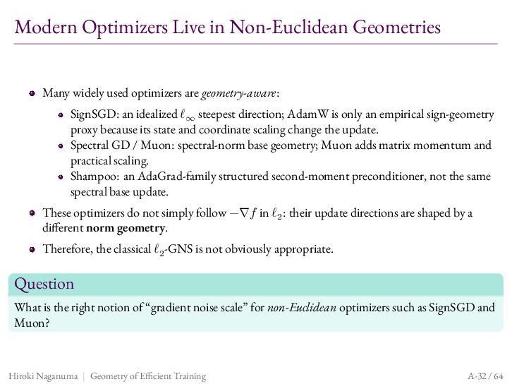
83. Modern Optimizers Live in Non-Euclidean Geometries Many widely used optimizers are geometry-aware: SignSGD: an idealized ℓ∞ steepest direction; AdamW is only an empirical sign-geometry proxy because its state and coordinate scaling change the update. Spectral GD / Muon: spectral-norm base geometry; Muon adds matrix momentum and practical scaling. Shampoo: an AdaGrad-family structured second-moment preconditioner, not the same spectral base update. These optimizers do not simply follow −∇𝑓 in ℓ2 : their update directions are shaped by a different norm geometry. Therefore, the classical ℓ2 -GNS is not obviously appropriate. Question What is the right notion of “gradient noise scale” for non-Euclidean optimizers such as SignSGD and Muon? Hiroki Naganuma | Geometry of Efficient Training A-32 / 64
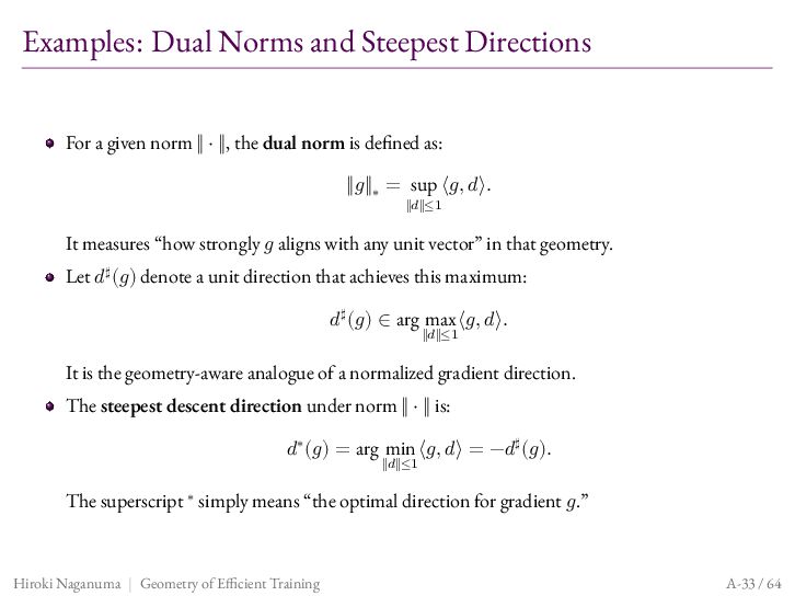
84. Examples: Dual Norms and Steepest Directions For a given norm ‖ ⋅ ‖, the dual norm is defined as: ‖𝑔‖∗ = sup ⟨𝑔, 𝑑⟩. ‖𝑑‖≤1 It measures “how strongly 𝑔 aligns with any unit vector” in that geometry. Let 𝑑♯ (𝑔) denote a unit direction that achieves this maximum: 𝑑♯ (𝑔) ∈ arg max ⟨𝑔, 𝑑⟩. ‖𝑑‖≤1 It is the geometry-aware analogue of a normalized gradient direction. The steepest descent direction under norm ‖ ⋅ ‖ is: 𝑑∗ (𝑔) = arg min ⟨𝑔, 𝑑⟩ = −𝑑♯ (𝑔). ‖𝑑‖≤1 The superscript ∗ simply means “the optimal direction for gradient 𝑔.” Hiroki Naganuma | Geometry of Efficient Training A-33 / 64
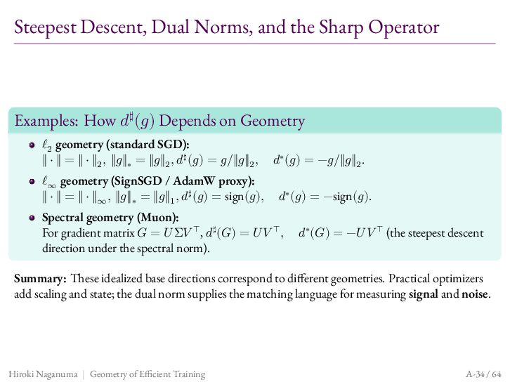
85. Steepest Descent, Dual Norms, and the Sharp Operator Examples: How 𝑑♯ (𝑔) Depends on Geometry ℓ2 geometry (standard SGD): ‖ ⋅ ‖ = ‖ ⋅ ‖2 , ‖𝑔‖∗ = ‖𝑔‖2 , 𝑑♯ (𝑔) = 𝑔/‖𝑔‖2 , 𝑑∗ (𝑔) = −𝑔/‖𝑔‖2 . ℓ∞ geometry (SignSGD / AdamW proxy): ‖ ⋅ ‖ = ‖ ⋅ ‖∞ , ‖𝑔‖∗ = ‖𝑔‖1 , 𝑑♯ (𝑔) = sign(𝑔), 𝑑∗ (𝑔) = −sign(𝑔). Spectral geometry (Muon): For gradient matrix 𝐺 = 𝑈 Σ𝑉 ⊤ , 𝑑♯ (𝐺) = 𝑈 𝑉 ⊤ , direction under the spectral norm). 𝑑∗ (𝐺) = −𝑈 𝑉 ⊤ (the steepest descent Summary: These idealized base directions correspond to different geometries. Practical optimizers add scaling and state; the dual norm supplies the matching language for measuring signal and noise. Hiroki Naganuma | Geometry of Efficient Training A-34 / 64
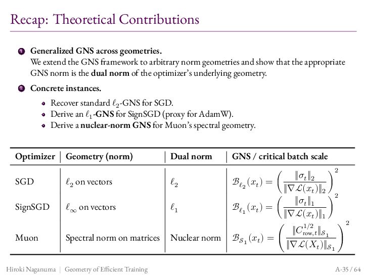
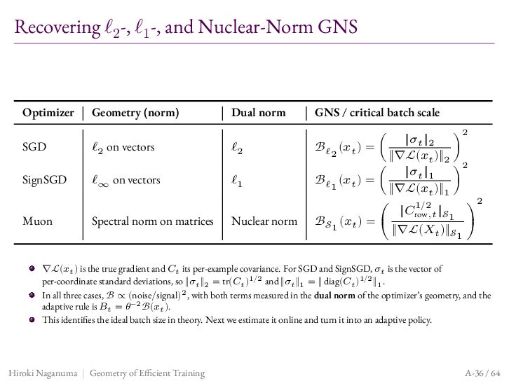
86. Recap: Theoretical Contributions 1 2 Generalized GNS across geometries. We extend the GNS framework to arbitrary norm geometries and show that the appropriate GNS norm is the dual norm of the optimizer’s underlying geometry. Concrete instances. Recover standard ℓ2 -GNS for SGD. Derive an ℓ1 -GNS for SignSGD (proxy for AdamW). Derive a nuclear-norm GNS for Muon’s spectral geometry. Optimizer Geometry (norm) Dual norm GNS / critical batch scale SGD ℓ2 on vectors ℓ2 ℬℓ2 (𝑥𝑡 ) = ( SignSGD ℓ∞ on vectors ℓ1 2 ‖𝜎𝑡 ‖2 ) ‖∇ℒ(𝑥𝑡 )‖2 2 ‖𝜎𝑡 ‖1 ℬℓ1 (𝑥𝑡 ) = ( ) ‖∇ℒ(𝑥𝑡 )‖1 1/2 Muon Spectral norm on matrices Hiroki Naganuma | Geometry of Efficient Training Nuclear norm 2 ‖𝐶row,𝑡 ‖𝒮1 ℬ𝒮1 (𝑥𝑡 ) = ( ) ‖∇ℒ(𝑋𝑡 )‖𝒮1 A-35 / 64
87. Recovering ℓ2 -, ℓ1 -, and Nuclear-Norm GNS Optimizer Geometry (norm) Dual norm GNS / critical batch scale SGD ℓ2 on vectors ℓ2 ℬℓ2 (𝑥𝑡 ) = ( SignSGD ℓ∞ on vectors ℓ1 2 ‖𝜎𝑡 ‖2 ) ‖∇ℒ(𝑥𝑡 )‖2 2 ‖𝜎𝑡 ‖1 ℬℓ1 (𝑥𝑡 ) = ( ) ‖∇ℒ(𝑥𝑡 )‖1 1/2 Muon Spectral norm on matrices Nuclear norm 2 ‖𝐶row,𝑡 ‖𝒮1 ⎞ ⎜ ⎟ ℬ𝒮1 (𝑥𝑡 ) = ⎛ ‖∇ℒ(𝑋𝑡 )‖𝒮1 ⎝ ⎠ ∇ℒ(𝑥𝑡 ) is the true gradient and 𝐶𝑡 its per-example covariance. For SGD and SignSGD, 𝜎𝑡 is the vector of per-coordinate standard deviations, so ‖𝜎𝑡 ‖2 = tr(𝐶𝑡 )1/2 and ‖𝜎𝑡 ‖1 = ‖ diag(𝐶𝑡 )1/2 ‖1 . In all three cases, ℬ ∝ (noise/signal)2 , with both terms measured in the dual norm of the optimizer’s geometry, and the adaptive rule is 𝐵𝑡 = 𝜃−2 ℬ(𝑥𝑡 ). This identifies the ideal batch size in theory. Next we estimate it online and turn it into an adaptive policy. Hiroki Naganuma | Geometry of Efficient Training A-36 / 64
88. Example: ℓ1 -GNS for SignSGD Consider SignSGD [3] with update 𝑥𝑡+1 = 𝑥𝑡 − 𝜂𝑡 sign(𝑔𝑡 ), where 𝑔𝑡 is the mini-batch gradient. Using a second-order Taylor expansion and expectations over mini-batches (with 𝔼𝑡 [‖∇ℒ(𝑥𝑡 ) − 𝑔𝑡 ‖1 ] ≤ ‖𝜎𝑡 ‖1 /√𝐵𝑡 ), we bound the expected loss reduction as 𝑡 ‖1 )− 𝔼[Δℒ](𝜂𝑡 , 𝐵𝑡 ) ≳ 𝜂𝑡 (‖∇ℒ(𝑥𝑡 )‖1 − ‖𝜎 √𝐵 𝑡 𝑀 𝜂𝑡2 . 2 Optimizing over the learning rate and extracting the “turning point” in 𝐵𝑡 yields the ℓ1 -GNS: ℬℓ1 (𝑥𝑡 ) = ‖𝜎𝑡 ‖21 , ‖∇ℒ(𝑥𝑡 )‖21 ‖𝜎𝑡 ‖1 = ‖ diag(𝐶𝑡 )1/2 ‖1 . This plays the same role as ℓ2 -GNS for SGD, but now aligned with SignSGD’s underlying geometry (and serves as a proxy for AdamW). Hiroki Naganuma | Geometry of Efficient Training A-37 / 64
89. Example: Nuclear-Norm GNS for Muon For Muon [11], each update uses the matrix gradient 𝐺𝑡 with SVD 𝐺𝑡 = 𝑈 diag(𝜎) 𝑉 ⊤ and matrix sign matsign(𝐺𝑡 ) = 𝑈 𝑉 ⊤ . The spectral steepest-descent step is proportional to −𝑈 𝑉 ⊤ , so the alignment between ∇ℒ(𝑋𝑡 ) and the update is controlled by the nuclear (𝒮1 ) norm: ‖∇ℒ(𝑋𝑡 )‖𝒮1 = ∑ 𝜎𝑖 (∇ℒ(𝑋𝑡 )). 𝑖 1/2 The noise term depends on ‖𝐶row,𝑡 ‖𝒮1 , the nuclear norm of the per-example gradient noise. The resulting critical batch size again has the form 1/2 ℬ𝒮1 (𝑥𝑡 ) = ( ‖𝐶row,𝑡 ‖𝒮1 2 ) , ‖∇ℒ(𝑋𝑡 )‖𝒮1 which matches the intuition that Muon is operating in spectral geometry. Hiroki Naganuma | Geometry of Efficient Training A-38 / 64
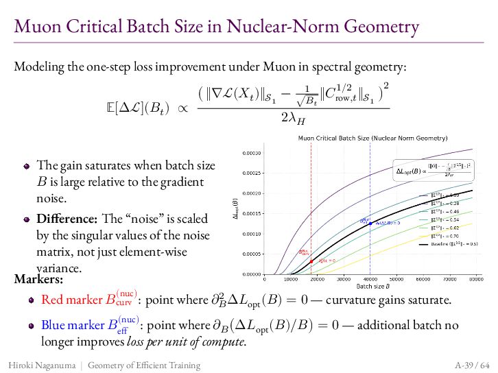
90. Muon Critical Batch Size in Nuclear-Norm Geometry Modeling the one-step loss improvement under Muon in spectral geometry: 1/2 𝔼[Δℒ](𝐵𝑡 ) ∝ 1 ‖𝐶row,𝑡 ‖𝒮1 ) ( ‖∇ℒ(𝑋𝑡 )‖𝒮1 − √𝐵 2 𝑡 2𝜆𝐻 The gain saturates when batch size 𝐵 is large relative to the gradient noise. Difference: The “noise” is scaled by the singular values of the noise matrix, not just element-wise variance. Markers: (nuc) 2 Red marker 𝐵curv : point where 𝜕𝐵 Δ𝐿opt (𝐵) = 0 — curvature gains saturate. (nuc) Blue marker 𝐵eff : point where 𝜕𝐵 (Δ𝐿opt (𝐵)/𝐵) = 0 — additional batch no longer improves loss per unit of compute. Hiroki Naganuma | Geometry of Efficient Training A-39 / 64
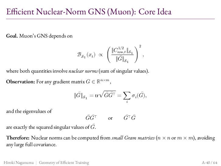
91. Efficient Nuclear-Norm GNS (Muon): Core Idea Goal. Muon’s GNS depends on 2 1/2 ‖𝐶row,𝑡 ‖𝒮1 ℬ𝒮1 (𝑥𝑡 ) ∝ ( ) , ‖𝐺‖̄ 𝒮1 where both quantities involve nuclear norms (sum of singular values). Observation: For any gradient matrix 𝐺 ∈ ℝ𝑛×𝑚 , ̄ ⊤̄ = ∑ 𝜎 (𝐺), ̄ ‖𝐺‖̄ 𝒮1 = tr√𝐺𝐺 𝑖 𝑖 and the eigenvalues of ̄ ⊤̄ 𝐺𝐺 are exactly the squared singular values of 𝐺.̄ or 𝐺⊤̄ 𝐺 ̄ Therefore: Nuclear norms can be computed from small Gram matrices (𝑛 × 𝑛 or 𝑚 × 𝑚), avoiding any large full covariance. Hiroki Naganuma | Geometry of Efficient Training A-40 / 64
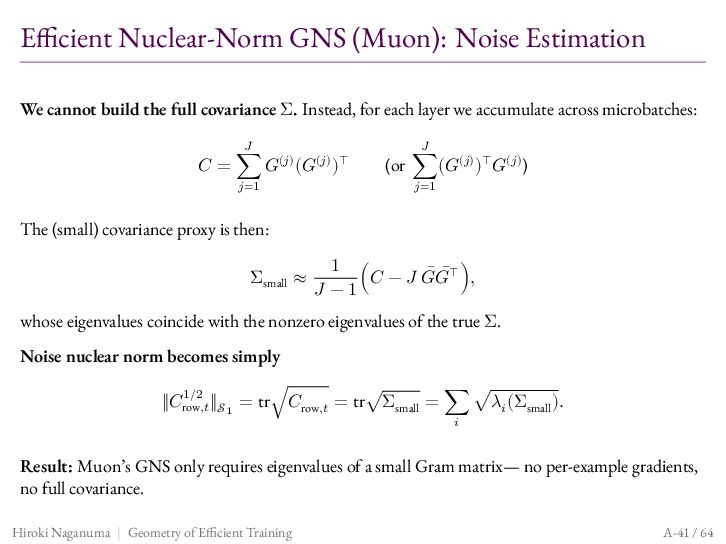
92. Efficient Nuclear-Norm GNS (Muon): Noise Estimation We cannot build the full covariance Σ. Instead, for each layer we accumulate across microbatches: 𝐽 𝐽 𝐶 = ∑ 𝐺(𝑗) (𝐺(𝑗) )⊤ 𝑗=1 (or ∑(𝐺(𝑗) )⊤ 𝐺(𝑗) ) 𝑗=1 The (small) covariance proxy is then: Σsmall ≈ 1 ̄ ⊤̄ ), (𝐶 − 𝐽 𝐺𝐺 𝐽 −1 whose eigenvalues coincide with the nonzero eigenvalues of the true Σ. Noise nuclear norm becomes simply 1/2 ‖𝐶row,𝑡 ‖𝒮1 = tr√𝐶row,𝑡 = tr√Σsmall = ∑ √𝜆𝑖 (Σsmall ). 𝑖 Result: Muon’s GNS only requires eigenvalues of a small Gram matrix— no per-example gradients, no full covariance. Hiroki Naganuma | Geometry of Efficient Training A-41 / 64
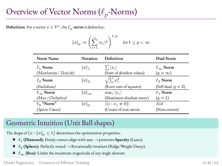
93. Overview of Vector Norms (ℓ𝑝 -Norms) Definition: For a vector 𝑥 ∈ ℝ𝑛 , the ℓ𝑝 -norm is defined as: 𝑛 1/𝑝 ‖𝑥‖𝑝 ∶= (∑ |𝑥𝑖 |𝑝 ) for 1 ≤ 𝑝 < ∞ 𝑖=1 Norm Name Notation Definition Dual Norm ℓ1 Norm (Manhattan / Taxicab) ‖𝑥‖1 ∑ |𝑥𝑖 | (Sum of absolute values) ℓ∞ Norm (𝑞 = ∞) ℓ2 Norm ‖𝑥‖2 √∑ 𝑥2𝑖 ℓ2 Norm (Root sum of squares) max𝑖 |𝑥𝑖 | (Maximum absolute entry) |{𝑖 ∶ 𝑥𝑖 ≠ 0}| (Count of non-zeros) (Self-dual, 𝑞 = 2) ℓ1 Norm (𝑞 = 1) N/A (Non-convex) (Euclidean) ℓ∞ Norm (Max / Chebyshev) ℓ0 “Norm” (Sparse Count) ‖𝑥‖∞ ‖𝑥‖0 Geometric Intuition (Unit Ball shapes) The shape of {𝑥 ∶ ‖𝑥‖𝑝 ≤ 1} determines the optimization properties: ℓ1 (Diamond): Pointy corners align with axes → promotes Sparsity (Lasso). ℓ2 (Sphere): Perfectly round → Rotationally invariant (Ridge/Weight Decay). ℓ∞ (Box): Limits the maximum magnitude of any single element. Hiroki Naganuma | Geometry of Efficient Training A-42 / 64
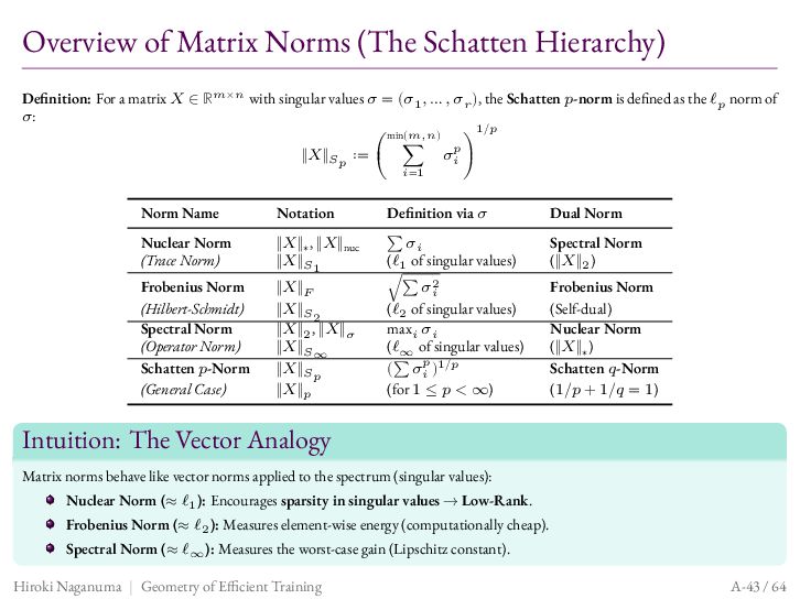
94. Overview of Matrix Norms (The Schatten Hierarchy) Definition: For a matrix 𝑋 ∈ ℝ𝑚×𝑛 with singular values 𝜎 = (𝜎1 , … , 𝜎𝑟 ), the Schatten 𝑝-norm is defined as the ℓ𝑝 norm of 𝜎: min(𝑚,𝑛) ⎜ ‖𝑋‖𝑆𝑝 ∶= ⎛ ⎝ ∑ 𝑖=1 1/𝑝 ⎟ 𝜎𝑖𝑝 ⎞ ⎠ Norm Name Notation Definition via 𝜎 Dual Norm Nuclear Norm (Trace Norm) ‖𝑋‖∗ , ‖𝑋‖nuc ‖𝑋‖𝑆1 ∑ 𝜎𝑖 (ℓ1 of singular values) Spectral Norm (‖𝑋‖2 ) Frobenius Norm (Hilbert-Schmidt) Spectral Norm (Operator Norm) Schatten 𝑝-Norm (General Case) ‖𝑋‖𝐹 ‖𝑋‖𝑆2 ‖𝑋‖2 , ‖𝑋‖𝜎 ‖𝑋‖𝑆∞ ‖𝑋‖𝑆𝑝 ‖𝑋‖𝑝 √∑ 𝜎𝑖2 (ℓ2 of singular values) max𝑖 𝜎𝑖 (ℓ∞ of singular values) (∑ 𝜎𝑖𝑝 )1/𝑝 (for 1 ≤ 𝑝 < ∞) Frobenius Norm (Self-dual) Nuclear Norm (‖𝑋‖∗ ) Schatten 𝑞-Norm (1/𝑝 + 1/𝑞 = 1) Intuition: The Vector Analogy Matrix norms behave like vector norms applied to the spectrum (singular values): Nuclear Norm (≈ ℓ1 ): Encourages sparsity in singular values → Low-Rank. Frobenius Norm (≈ ℓ2 ): Measures element-wise energy (computationally cheap). Spectral Norm (≈ ℓ∞ ): Measures the worst-case gain (Lipschitz constant). Hiroki Naganuma | Geometry of Efficient Training A-43 / 64
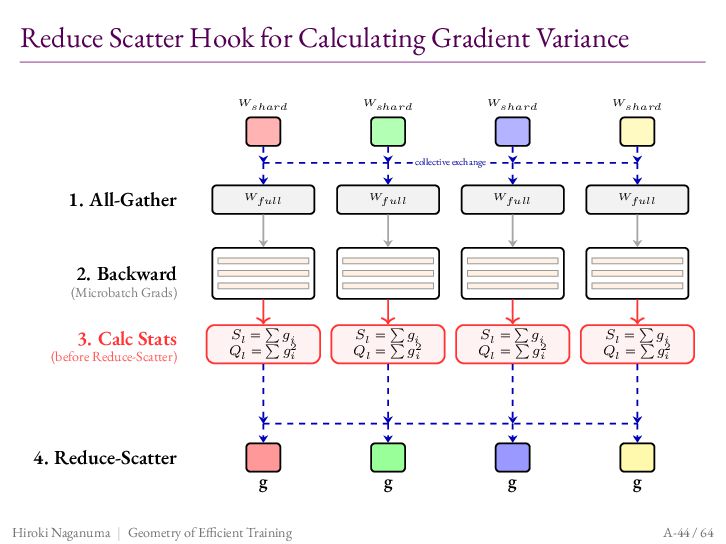
95. Reduce Scatter Hook for Calculating Gradient Variance 𝑊𝑠ℎ𝑎𝑟𝑑 𝑊𝑠ℎ𝑎𝑟𝑑 𝑊𝑠ℎ𝑎𝑟𝑑 𝑊𝑠ℎ𝑎𝑟𝑑 collective exchange 1. All-Gather 𝑊𝑓𝑢𝑙𝑙 𝑊𝑓𝑢𝑙𝑙 𝑊𝑓𝑢𝑙𝑙 𝑊𝑓𝑢𝑙𝑙 𝑆𝑙 = ∑ 𝑔 𝑖 𝑄𝑙 = ∑ 𝑔𝑖2 𝑆𝑙 = ∑ 𝑔 𝑖 𝑄𝑙 = ∑ 𝑔𝑖2 𝑆𝑙 = ∑ 𝑔 𝑖 𝑄𝑙 = ∑ 𝑔𝑖2 𝑆𝑙 = ∑ 𝑔 𝑖 𝑄𝑙 = ∑ 𝑔𝑖2 g g g g 2. Backward (Microbatch Grads) 3. Calc Stats (before Reduce-Scatter) 4. Reduce-Scatter Hiroki Naganuma | Geometry of Efficient Training A-44 / 64
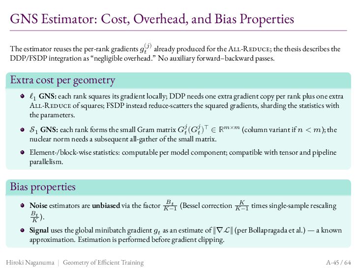
96. GNS Estimator: Cost, Overhead, and Bias Properties (𝑗) The estimator reuses the per-rank gradients 𝑔𝑡 already produced for the All-Reduce; the thesis describes the DDP/FSDP integration as “negligible overhead.” No auxiliary forward–backward passes. Extra cost per geometry ℓ1 GNS: each rank squares its gradient locally; DDP needs one extra gradient copy per rank plus one extra All-Reduce of squares; FSDP instead reduce-scatters the squared gradients, sharding the statistics with the parameters. 𝒮1 GNS: each rank forms the small Gram matrix 𝐺𝑗𝑡 (𝐺𝑗𝑡 )⊤ ∈ ℝ𝑚×𝑚 (column variant if 𝑛 < 𝑚); the nuclear norm needs a subsequent all-gather of the small matrix. Element-/block-wise statistics: computable per model component; compatible with tensor and pipeline parallelism. Bias properties 𝐵𝑡 𝐾 Noise estimators are unbiased via the factor 𝐾−1 (Bessel correction 𝐾−1 times single-sample rescaling 𝐵𝑡 ). 𝐾 Signal uses the global minibatch gradient 𝑔𝑡 as an estimate of ‖∇ℒ‖ (per Bollapragada et al.) — a known approximation. Estimation is performed before gradient clipping. Hiroki Naganuma | Geometry of Efficient Training A-45 / 64
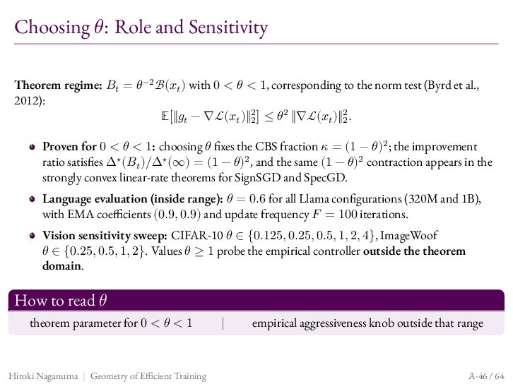
97. Choosing 𝜃: Role and Sensitivity Theorem regime: 𝐵𝑡 = 𝜃−2 ℬ(𝑥𝑡 ) with 0 < 𝜃 < 1, corresponding to the norm test (Byrd et al., 2012): 𝔼[‖𝑔𝑡 − ∇ℒ(𝑥𝑡 )‖22 ] ≤ 𝜃2 ‖∇ℒ(𝑥𝑡 )‖22 . Proven for 0 < 𝜃 < 1: choosing 𝜃 fixes the CBS fraction 𝜅 = (1 − 𝜃)2 ; the improvement ratio satisfies Δ⋆ (𝐵𝑡 )/Δ⋆ (∞) = (1 − 𝜃)2 , and the same (1 − 𝜃)2 contraction appears in the strongly convex linear-rate theorems for SignSGD and SpecGD. Language evaluation (inside range): 𝜃 = 0.6 for all Llama configurations (320M and 1B), with EMA coefficients (0.9, 0.9) and update frequency 𝐹 = 100 iterations. Vision sensitivity sweep: CIFAR-10 𝜃 ∈ {0.125, 0.25, 0.5, 1, 2, 4}, ImageWoof 𝜃 ∈ {0.25, 0.5, 1, 2}. Values 𝜃 ≥ 1 probe the empirical controller outside the theorem domain. How to read 𝜃 theorem parameter for 0 < 𝜃 < 1 Hiroki Naganuma | Geometry of Efficient Training | empirical aggressiveness knob outside that range A-46 / 64
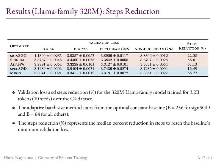
98. Results (Llama-family 320M): Steps Reduction Validation loss and steps reduction (%) for the 320M Llama-family model trained for 3.2B tokens (10 seeds) over the C4 dataset. The adaptive batch size method starts from the optimal constant baseline (B = 256 for signSGD and B = 64 for all others). The steps reduction (%) represents the median percent reduction in steps to reach the baseline’s minimum validation loss. Hiroki Naganuma | Geometry of Efficient Training A-47 / 64
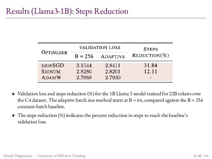
99. Results (Llama3-1B): Steps Reduction Validation loss and steps reduction (%) for the 1B Llama 3 model trained for 22B tokens over the C4 dataset. The adaptive batch size method starts at B = 64, compared against the B = 256 constant-batch baseline. The steps reduction (%) indicates the percent reduction in steps to reach the baseline’s validation loss. Hiroki Naganuma | Geometry of Efficient Training A-48 / 64
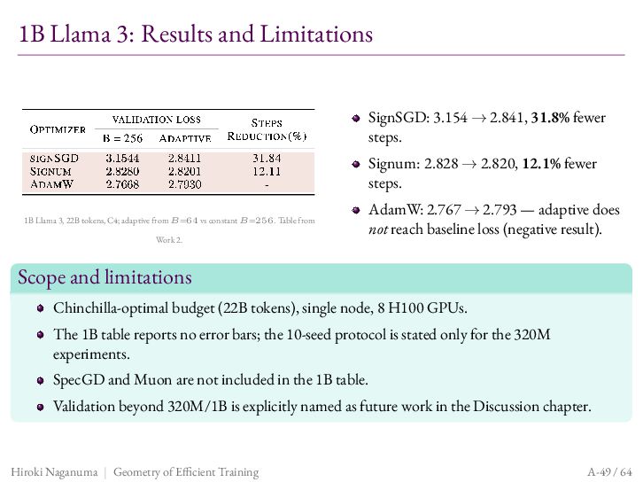
100. 1B Llama 3: Results and Limitations SignSGD: 3.154 → 2.841, 31.8% fewer steps. Signum: 2.828 → 2.820, 12.1% fewer steps. 1B Llama 3, 22B tokens, C4; adaptive from 𝐵=64 vs constant 𝐵=256. Table from Work 2. AdamW: 2.767 → 2.793 — adaptive does not reach baseline loss (negative result). Scope and limitations Chinchilla-optimal budget (22B tokens), single node, 8 H100 GPUs. The 1B table reports no error bars; the 10-seed protocol is stated only for the 320M experiments. SpecGD and Muon are not included in the 1B table. Validation beyond 320M/1B is explicitly named as future work in the Discussion chapter. Hiroki Naganuma | Geometry of Efficient Training A-49 / 64
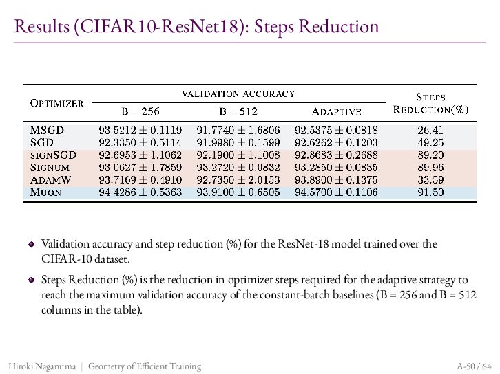
101. Results (CIFAR10-ResNet18): Steps Reduction Validation accuracy and step reduction (%) for the ResNet-18 model trained over the CIFAR-10 dataset. Steps Reduction (%) is the reduction in optimizer steps required for the adaptive strategy to reach the maximum validation accuracy of the constant-batch baselines (B = 256 and B = 512 columns in the table). Hiroki Naganuma | Geometry of Efficient Training A-50 / 64
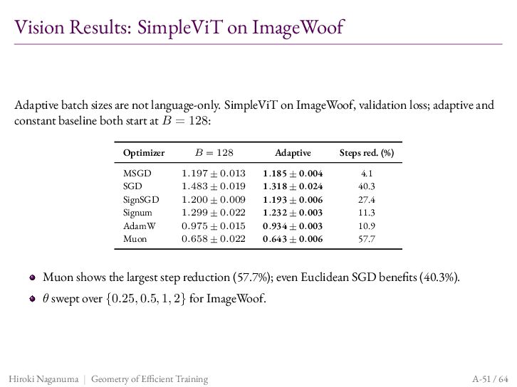
102. Vision Results: SimpleViT on ImageWoof Adaptive batch sizes are not language-only. SimpleViT on ImageWoof, validation loss; adaptive and constant baseline both start at 𝐵 = 128: Optimizer 𝐵 = 128 Adaptive Steps red. (%) MSGD SGD SignSGD Signum AdamW Muon 1.197 ± 0.013 1.483 ± 0.019 1.200 ± 0.009 1.299 ± 0.022 0.975 ± 0.015 0.658 ± 0.022 1.185 ± 0.004 1.318 ± 0.024 1.193 ± 0.006 1.232 ± 0.003 0.934 ± 0.003 0.643 ± 0.006 4.1 40.3 27.4 11.3 10.9 57.7 Muon shows the largest step reduction (57.7%); even Euclidean SGD benefits (40.3%). 𝜃 swept over {0.25, 0.5, 1, 2} for ImageWoof. Hiroki Naganuma | Geometry of Efficient Training A-51 / 64
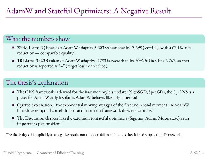
103. AdamW and Stateful Optimizers: A Negative Result What the numbers show 320M Llama 3 (10 seeds): AdamW adaptive 3.303 vs best baseline 3.299 (𝐵=64), with a 67.1% step reduction — comparable quality. 1B Llama 3 (22B tokens): AdamW adaptive 2.793 is worse than its 𝐵=256 baseline 2.767, so step reduction is reported as “–” (target loss not reached). The thesis’s explanation The GNS framework is derived for the base memoryless updates (SignSGD, SpecGD); the ℓ1 GNS is a proxy for AdamW only insofar as AdamW behaves like a sign method. Quoted explanation: “the exponential moving averages of the first and second moments in AdamW introduce temporal correlations that our current framework does not capture.” The Discussion chapter lists the extension to stateful optimizers (Signum, Adam, Muon state) as an important open problem. The thesis flags this explicitly as a negative result, not a hidden failure; it bounds the claimed scope of the framework. Hiroki Naganuma | Geometry of Efficient Training A-52 / 64
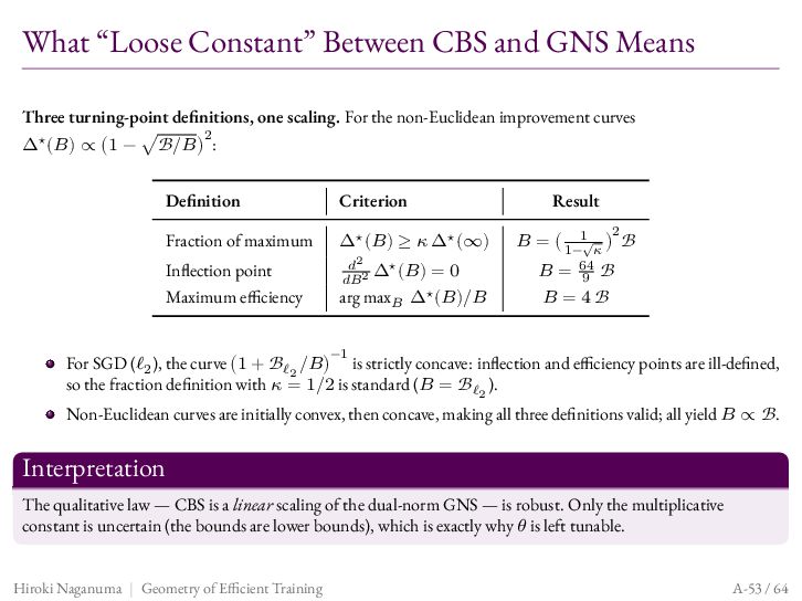
104. What “Loose Constant” Between CBS and GNS Means Three turning-point definitions, one scaling. For the non-Euclidean improvement curves 2 Δ⋆ (𝐵) ∝ (1 − √ℬ/𝐵) : Definition Criterion Fraction of maximum Δ⋆ (𝐵) ≥ 𝜅 Δ⋆ (∞) Inflection point 𝑑2 𝑑𝐵2 Maximum efficiency Result Δ⋆ (𝐵) = 0 arg max𝐵 Δ⋆ (𝐵)/𝐵 2 𝐵 = ( 1−1√𝜅 ) ℬ 𝐵 = 64 9 ℬ 𝐵 = 4ℬ −1 For SGD (ℓ2 ), the curve (1 + ℬℓ2 /𝐵) is strictly concave: inflection and efficiency points are ill-defined, so the fraction definition with 𝜅 = 1/2 is standard (𝐵 = ℬℓ2 ). Non-Euclidean curves are initially convex, then concave, making all three definitions valid; all yield 𝐵 ∝ ℬ. Interpretation The qualitative law — CBS is a linear scaling of the dual-norm GNS — is robust. Only the multiplicative constant is uncertain (the bounds are lower bounds), which is exactly why 𝜃 is left tunable. Hiroki Naganuma | Geometry of Efficient Training A-53 / 64
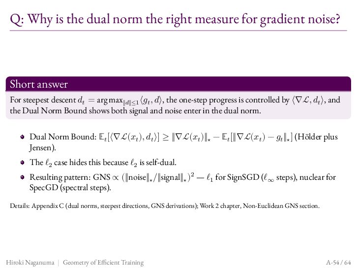
105. Q: Why is the dual norm the right measure for gradient noise? Short answer For steepest descent 𝑑𝑡 = arg max‖𝑑‖≤1 ⟨𝑔𝑡 , 𝑑⟩, the one-step progress is controlled by ⟨∇ℒ, 𝑑𝑡 ⟩, and the Dual Norm Bound shows both signal and noise enter in the dual norm. Dual Norm Bound: 𝔼𝑡 [⟨∇ℒ(𝑥𝑡 ), 𝑑𝑡 ⟩] ≥ ‖∇ℒ(𝑥𝑡 )‖⋆ − 𝔼𝑡 [‖∇ℒ(𝑥𝑡 ) − 𝑔𝑡 ‖⋆ ] (Hölder plus Jensen). The ℓ2 case hides this because ℓ2 is self-dual. Resulting pattern: GNS ∝ (‖noise‖⋆ /‖signal‖⋆ )2 — ℓ1 for SignSGD (ℓ∞ steps), nuclear for SpecGD (spectral steps). Details: Appendix C (dual norms, steepest directions, GNS derivations); Work 2 chapter, Non-Euclidean GNS section. Hiroki Naganuma | Geometry of Efficient Training A-54 / 64
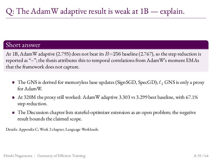
106. Q: The AdamW adaptive result is weak at 1B — explain. Short answer At 1B, AdamW adaptive (2.793) does not beat its 𝐵=256 baseline (2.767), so the step reduction is reported as “–”; the thesis attributes this to temporal correlations from AdamW’s moment EMAs that the framework does not capture. The GNS is derived for memoryless base updates (SignSGD, SpecGD); ℓ1 GNS is only a proxy for AdamW. At 320M the proxy still worked: AdamW adaptive 3.303 vs 3.299 best baseline, with 67.1% step reduction. The Discussion chapter lists stateful-optimizer extension as an open problem; the negative result bounds the claimed scope. Details: Appendix C; Work 2 chapter, Language Workloads. Hiroki Naganuma | Geometry of Efficient Training A-55 / 64
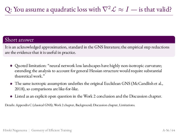
107. Q: You assume a quadratic loss with ∇2 ℒ ≈ 𝐼 — is that valid? Short answer It is an acknowledged approximation, standard in the GNS literature; the empirical step reductions are the evidence that it is useful in practice. Quoted limitation: “neural network loss landscapes have highly non-isotropic curvature; extending the analysis to account for general Hessian structure would require substantial theoretical work.” The same isotropic assumption underlies the original Euclidean GNS (McCandlish et al., 2018), so comparisons are like-for-like. Listed as an explicit open question in the Work 2 conclusion and the Discussion chapter. Details: Appendix C (classical GNS); Work 2 chapter, Background; Discussion chapter, Limitations. Hiroki Naganuma | Geometry of Efficient Training A-56 / 64
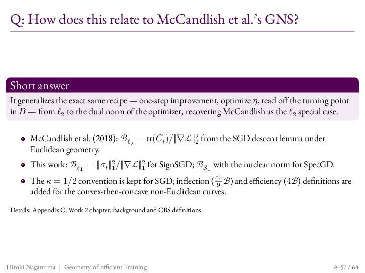
108. Q: How does this relate to McCandlish et al.’s GNS? Short answer It generalizes the exact same recipe — one-step improvement, optimize 𝜂, read off the turning point in 𝐵 — from ℓ2 to the dual norm of the optimizer, recovering McCandlish as the ℓ2 special case. McCandlish et al. (2018): ℬℓ2 = tr(𝐶𝑡 )/‖∇ℒ‖22 from the SGD descent lemma under Euclidean geometry. This work: ℬℓ1 = ‖𝜎𝑡 ‖21 /‖∇ℒ‖21 for SignSGD; ℬ𝒮1 with the nuclear norm for SpecGD. The 𝜅 = 1/2 convention is kept for SGD; inflection ( 64 ℬ) and efficiency (4ℬ) definitions are 9 added for the convex-then-concave non-Euclidean curves. Details: Appendix C; Work 2 chapter, Background and CBS definitions. Hiroki Naganuma | Geometry of Efficient Training A-57 / 64
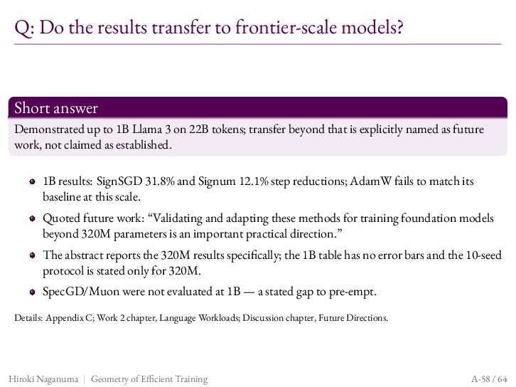
109. Q: Do the results transfer to frontier-scale models? Short answer Demonstrated up to 1B Llama 3 on 22B tokens; transfer beyond that is explicitly named as future work, not claimed as established. 1B results: SignSGD 31.8% and Signum 12.1% step reductions; AdamW fails to match its baseline at this scale. Quoted future work: “Validating and adapting these methods for training foundation models beyond 320M parameters is an important practical direction.” The abstract reports the 320M results specifically; the 1B table has no error bars and the 10-seed protocol is stated only for 320M. SpecGD/Muon were not evaluated at 1B — a stated gap to pre-empt. Details: Appendix C; Work 2 chapter, Language Workloads; Discussion chapter, Future Directions. Hiroki Naganuma | Geometry of Efficient Training A-58 / 64
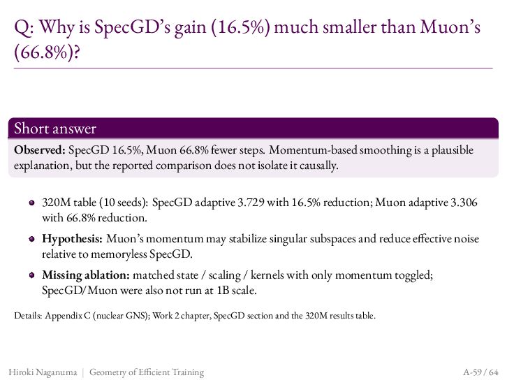
110. Q: Why is SpecGD’s gain (16.5%) much smaller than Muon’s (66.8%)? Short answer Observed: SpecGD 16.5%, Muon 66.8% fewer steps. Momentum-based smoothing is a plausible explanation, but the reported comparison does not isolate it causally. 320M table (10 seeds): SpecGD adaptive 3.729 with 16.5% reduction; Muon adaptive 3.306 with 66.8% reduction. Hypothesis: Muon’s momentum may stabilize singular subspaces and reduce effective noise relative to memoryless SpecGD. Missing ablation: matched state / scaling / kernels with only momentum toggled; SpecGD/Muon were also not run at 1B scale. Details: Appendix C (nuclear GNS); Work 2 chapter, SpecGD section and the 320M results table. Hiroki Naganuma | Geometry of Efficient Training A-59 / 64
111. Appendix D: Talk-Level Questions Cross-project questions: scope, publication status, and what is proven. Hiroki Naganuma | Geometry of Efficient Training A-60 / 64
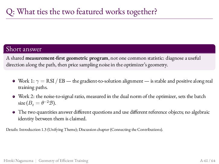
112. Q: What ties the two featured works together? Short answer A shared measurement-first geometric program, not one common statistic: diagnose a useful direction along the path, then price sampling noise in the optimizer’s geometry. Work 1: 𝛾 = RSI / EB — the gradient-to-solution alignment — is stable and positive along real training paths. Work 2: the noise-to-signal ratio, measured in the dual norm of the optimizer, sets the batch size (𝐵𝑡 = 𝜃−2 ℬ). The two quantities answer different questions and use different reference objects; no algebraic identity between them is claimed. Details: Introduction 1.3 (Unifying Theme); Discussion chapter (Connecting the Contributions). Hiroki Naganuma | Geometry of Efficient Training A-61 / 64
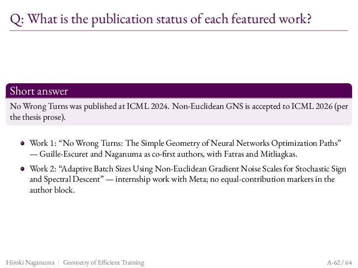
113. Q: What is the publication status of each featured work? Short answer No Wrong Turns was published at ICML 2024. Non-Euclidean GNS is accepted to ICML 2026 (per the thesis prose). Work 1: “No Wrong Turns: The Simple Geometry of Neural Networks Optimization Paths” — Guille-Escuret and Naganuma as co-first authors, with Fatras and Mitliagkas. Work 2: “Adaptive Batch Sizes Using Non-Euclidean Gradient Noise Scales for Stochastic Sign and Spectral Descent” — internship work with Meta; no equal-contribution markers in the author block. Hiroki Naganuma | Geometry of Efficient Training A-62 / 64
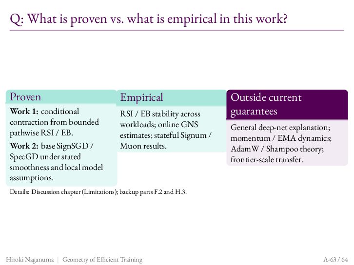
114. Q: What is proven vs. what is empirical in this work? Proven Empirical Work 1: conditional contraction from bounded pathwise RSI / EB. Work 2: base SignSGD / SpecGD under stated smoothness and local model assumptions. RSI / EB stability across workloads; online GNS estimates; stateful Signum / Muon results. Outside current guarantees General deep-net explanation; momentum / EMA dynamics; AdamW / Shampoo theory; frontier-scale transfer. Details: Discussion chapter (Limitations); backup parts F.2 and H.3. Hiroki Naganuma | Geometry of Efficient Training A-63 / 64
115. Q: How do No Wrong Turns’ 𝛾 and Non-Euclidean GNS relate? Short answer They are complementary diagnostics, not equivalent quantities. Large GNS does not by itself imply small 𝛾 without additional assumptions linking endpoint direction, mean gradient, and noise geometry. 𝛾: one sampled gradient vs. an endpoint direction. GNS: population signal vs. sampling variance in a chosen dual norm. Shared role: both expose when stochastic gradients remain useful; their empirical correlation is a testable hypothesis, not a theorem here. Details: Introduction 1.2 (Connection to other work, Non-Euclidean GNS subsection). Hiroki Naganuma | Geometry of Efficient Training A-64 / 64