Crouching Time Series, Hidden Markov Model: Applications of HMMs in the Real World

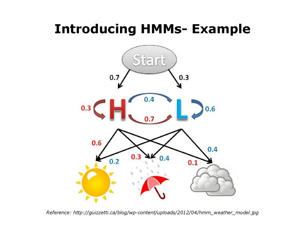
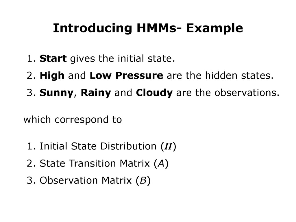
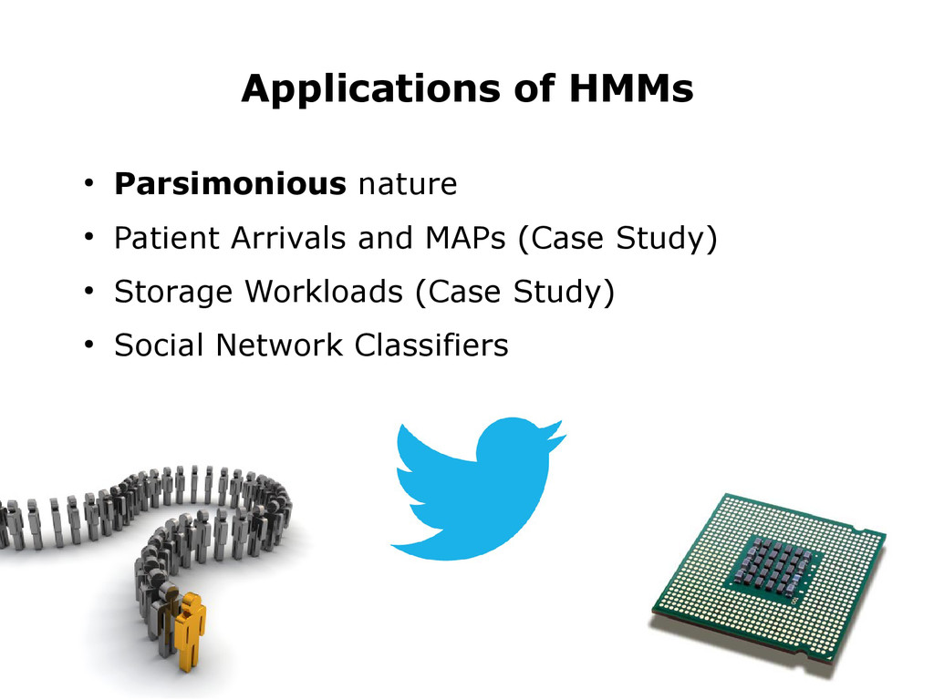
In this presentation, I will present an introduction and brief discussion into the applications and variations of the Hidden Markov Model (HMM), combining unsupervised learning techniques with performance analysis measures. Their parsimonious nature and efficient training on discrete and continuous data traces have made them popular as storage workloads, Markov Arrival Processes (MAPs), social network behaviour classifiers and financial predictive models (to name but a few). We explain relevant findings of the AESOP group (aesop.doc.ic.ac.uk/) over the last few years and mention possible future research.

Transcript

1. CROUCHING TIME SERIES HIDDEN MARKOV MODELS Applications of HMMs in the Real World Tiberiu Chis tiberiu.chis07@imperial.ac.uk AESOP Group
3. • Short Academic Bio • Introducing Hidden Markov Models (HMMs) • Applications of HMMs: Case Studies • Future Research • Tips Overview
4. Academic Bio • MSci in JMC (2007-11), UBS (2011-12), PhD (2012-?) • AESOP (Analysis, Engineering, Simulation & Optimization of Performance) Group
5. Introducing HMMs • Statistical Inference of Markov chains by Baum et al in late 1960s. • Speech recognition by Rabiner during 1970s. • Biological sequence analysis in late 1980s. • Storage Workload Modelling in 2000s. • many other applications.
6. Introducing HMMs- Example Reference: http://guizzetti.ca/blog/wp-content/uploads/2012/04/hmm_weather_model.jpg
7. Introducing HMMs- Example 1. Start gives the initial state. 2. High and Low Pressure are the hidden states. 3. Sunny, Rainy and Cloudy are the observations. which correspond to 1. Initial State Distribution (Π) 2. State Transition Matrix (A) 3. Observation Matrix (B)
8. • Parsimonious nature • Patient Arrivals and MAPs (Case Study) • Storage Workloads (Case Study) • Social Network Classifiers Applications of HMMs
9. • Observe Patients arriving at a Hospital • Transform Patient Arrivals data • HMM (MAP) training and prediction • Used for resource allocation and population monitoring Applications- Patient Arrivals
10. Raw trace Bin trace Obs trace Timestamped patient arrivals (i.e. 14:39) # of arrivals per hour (i.e. 4, 2, 0, 0, 5) Integer array with values between 1 and K Partition into one hour intervals K-means clustering algorithm Transform Patient Arrivals
11. Simulation of Patient Arrivals • 2 state model trained on 5000 data points. • 3 clusters for K-Means. • HMM parameters (Π, A, B) converge. • Synthetic observation trace is generated. • Simulate 1000 synthetic traces.
12. • Work published in LNEE • Proceedings of ISCIS 2013 (Paris) • “Analysing & Predicting Patient Arrival Times” Applications- Patient Arrivals
13. • Variations of HMM • Online Characterization of Workloads • Simulating Live Systems (i.e. Real time I/O requests and e-Commerce systems) • Avoid Resource Bottlenecks Applications- Storage Workloads
14. • Incremental HMM (IncHMM) • IncHMM parameters updated on the fly, improving time complexity of HMM • Accuracy of IncHMM matches HMM • Work published in LNCS • Proceedings of ASMTA 2013 (Ghent) • “iSWoM: Incremental Storage Workload Model” Applications- Storage Workloads
15. • Sliding HMM (SlidHMM) • Learning based on Moving Average • New data points replace old points • Work published in LNCS • Proceedings of EPEW 2013 (Venice) • “Sliding HMM for Evaluating Discrete Data” Applications- Storage Workloads
16. Training the SlidHMM HMM: 1 2 3 4 5 6 7 1 2 3 4 5 6 7 8 9 10 11 12 13 14 SlidHMM: 1 2 3 4 5 6 7 1 2 3 4 5 6 7 8 9 10 11 12 13 14
17. Training the SlidHMM HMM: 1 2 3 4 5 6 7 1 2 3 4 5 6 7 8 9 10 11 12 13 14 SlidHMM: 1 2 3 4 5 6 7 1 2 3 4 5 6 7 8 9 10 11 12 13 14
18. Training the SlidHMM HMM: 1 2 3 4 5 6 7 1 2 3 4 5 6 7 8 9 10 11 12 13 14 SlidHMM: 1 2 3 4 5 6 7 1 2 3 4 5 6 7 8 9 10 11 12 13 14
19. Benefits over HMM • IncHMM (and SlidHMM) have parameters which are updated on-the-fly: K is # of times that M new observations appear and T is size of original set S1 = steps taken to train HMM S2 = steps taken to train IncHMM
20. Benefits over HMM S1 = T + (T+M) + ... + (T+KM) = (K+1)T + ½K(K+1)M S2 = T + M + ... + M = T + KM S3 = S1 – S2 = K(T + ½(K-1)M)
21. • Model User Behaviour on Social Media • HMM behaves as a Workload Classifier of User Data • Parallel HMM for Multiple & Parallel Sessions Applications- Social Networks
22. • Parallel HMM uses Clustering to Group Points • Trains on Multiple Observations at once. • Improved HMM Convergence and Multi-User Temporal Activity Applications- Social Networks
23. • Financial Time Series Analysis and Stock Prediction • Continuous version of IncHMM and SlidHMM • Sports Modelling and Player Performance Evaluation Future Work with HMMs
24. • OK not to see your Supervisor often • Try to go to Talks and Conferences • Aim for Publications anywhere • Be present most days Tips