Did My Deploy Degrade Production?

Transcript

1. DID MY DEPLOY DEGRADE PRODUCTION? Ines Panker | Jun 2026 A SOLUTION WITHOUT AI
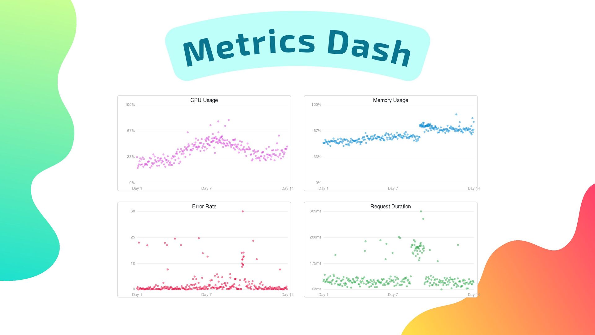
2. CPU Usage 0% 33% 67% 100% Day 1 Day 7 Day 14 Memory Usage 0% 33% 67% 100% Day 1 Day 7 Day 14 Error Rate 0 12 25 38 Day 1 Day 7 Day 14 Request Duration 63ms 172ms 280ms 389ms Day 1 Day 7 Day 14 Metrics Dash
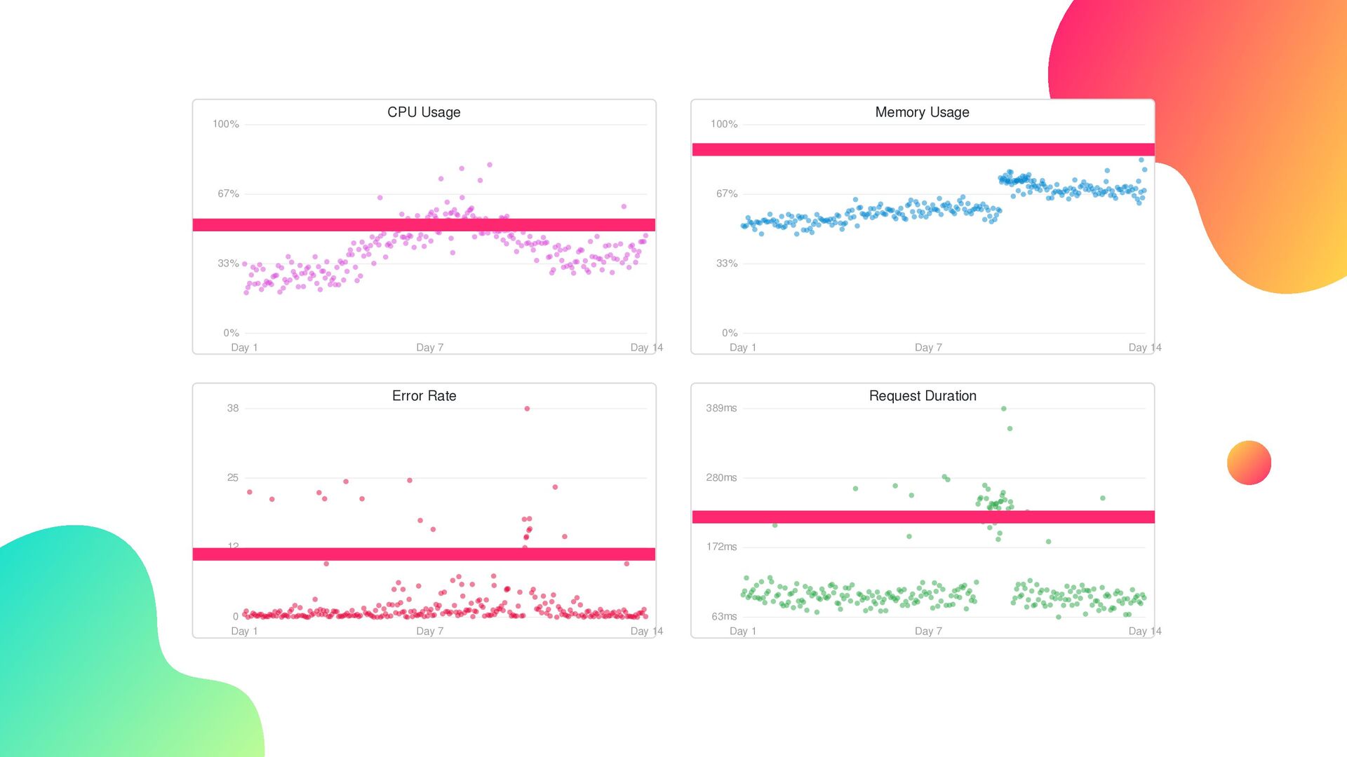
3. CPU Usage 0% 33% 67% 100% Day 1 Day 7 Day 14 Memory Usage 0% 33% 67% 100% Day 1 Day 7 Day 14 Error Rate 0 12 25 38 Day 1 Day 7 Day 14 Request Duration 63ms 172ms 280ms 389ms Day 1 Day 7 Day 14
4. 80 60 40 20 0 CPU (%) Jan Feb Mar Apr threshold start of change?
5. Automated Automated Health Health Detection Detection
7. and Quick Quick Quick Past Data Past Data Past Data ly analyze judge New Values New Values New Values
8. 2 2 2 Every mins
9. The Eternal Loop (every 2 minutes) Collect Metric (e.g., 142ms) Compare to Historical Data Return Health at least 14 days of history (10,080 data points)
10. HEALTHY :) all good AILING :/ hmm, watch UNHEALTHY :( ALERT
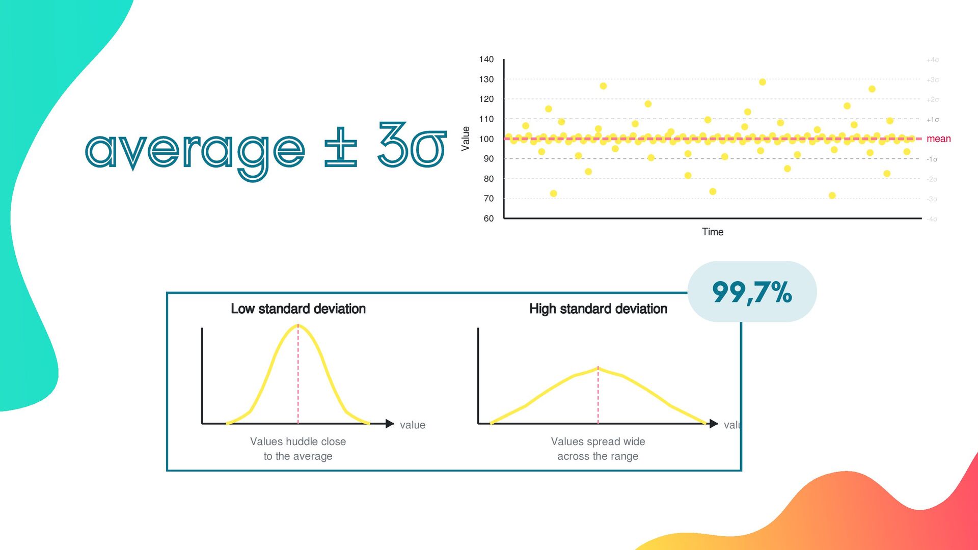
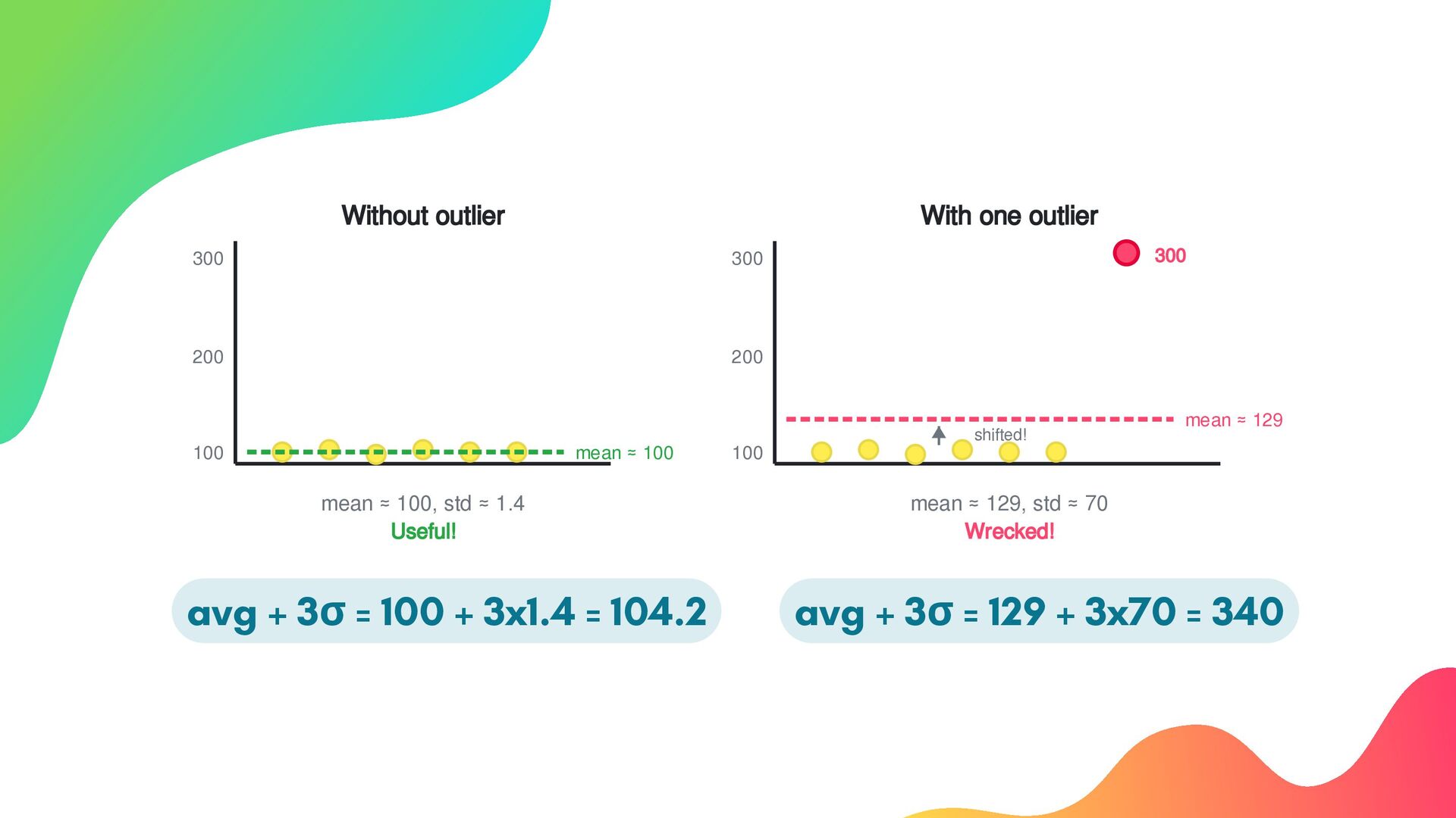
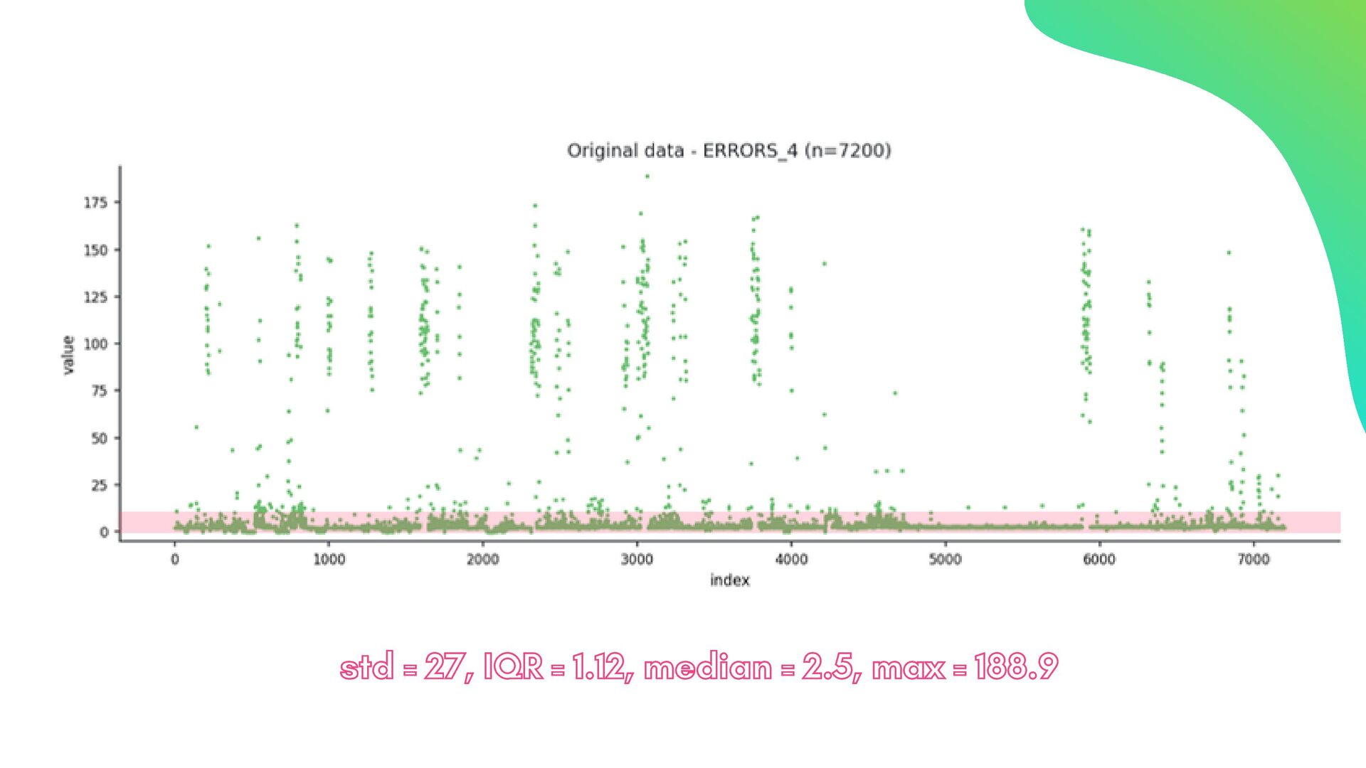
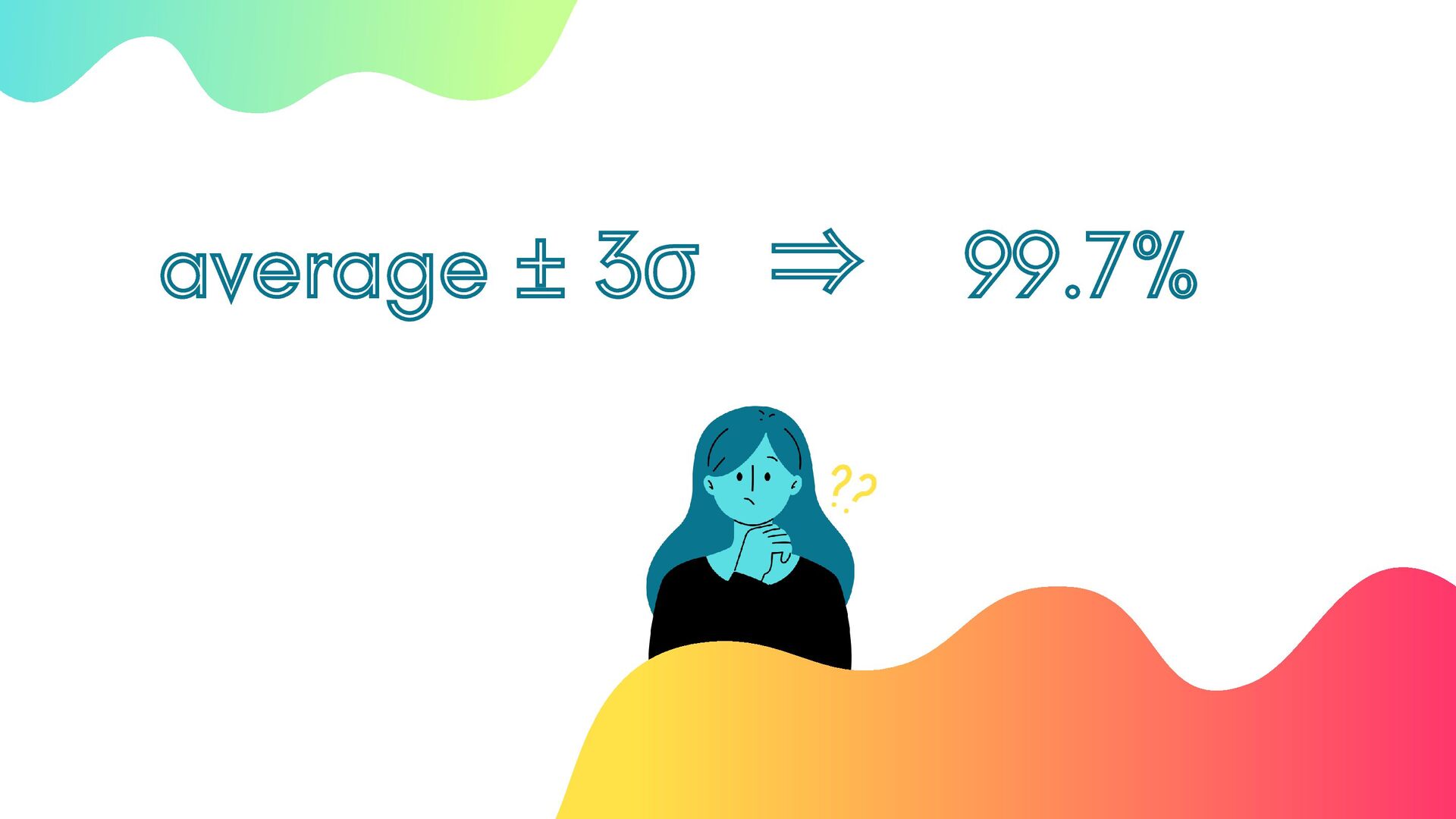
12. Low standard deviation value Values huddle close to the average High standard deviation valu Values spread wide across the range average ± 3σ average ± 3 σ 140 130 120 110 100 90 80 70 60 Value Time +1σ -1σ +2σ -2σ +3σ -3σ +4σ -4σ mean 99,7%
13. Without outlier 300 200 100 mean ≈ 100 mean ≈ 100, std ≈ 1.4 Useful! With one outlier 300 200 100 300 mean ≈ 129 shifted! mean ≈ 129, std ≈ 70 Wrecked! avg + 3σ = 100 + 3x1.4 = 104.2 avg + 3σ = 129 + 3x70 = 340
14. Day 1: Outlier detected normal values outlier! far away Day 5: Outliers are "normal" normal? neighbors! outliers became each other's k-nearest neighbors k-Nearest Neighbors k-Nearest Neighbors Outlier Detection Outlier Detection
15. Outliers Outliers Outliers Remove Remove Remove ...and then do statistics...
16. Major outliers Minor outliers KDE KDE KDE DBSCAN DBSCAN DBSCAN
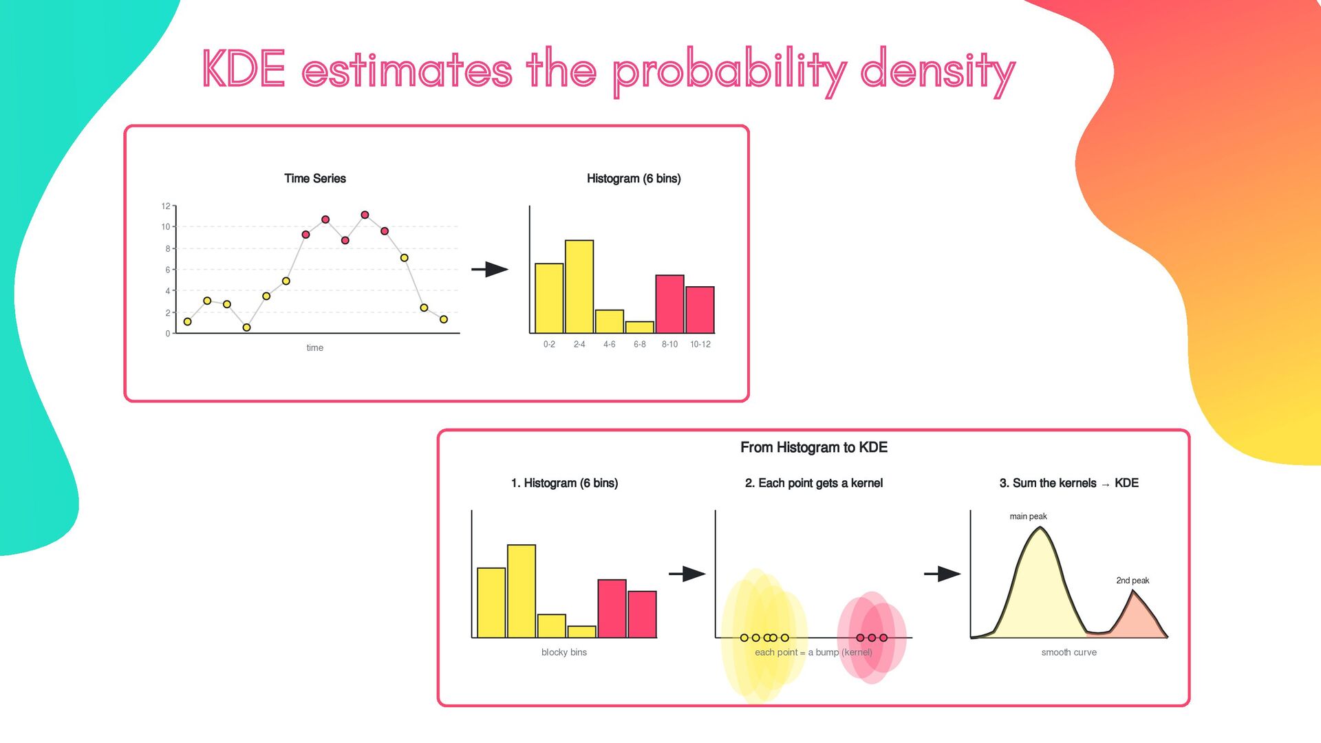
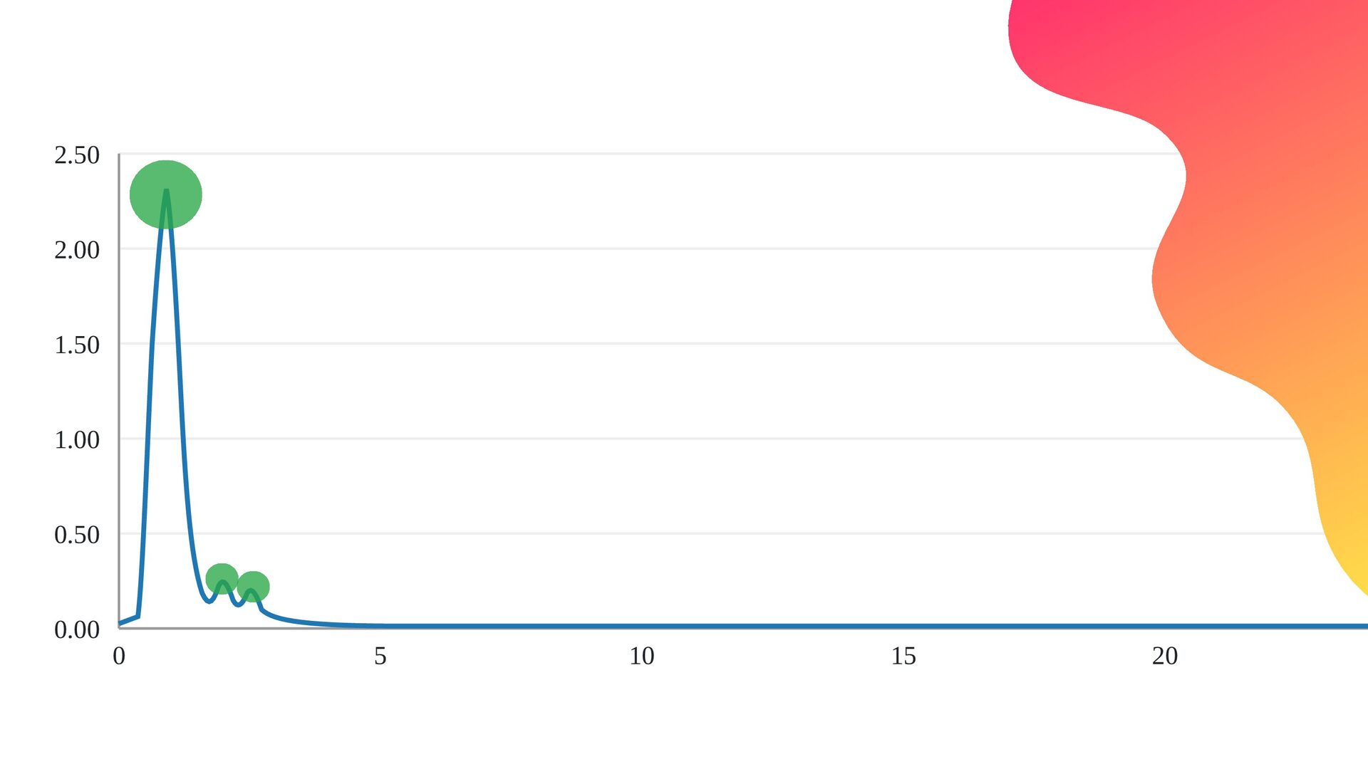
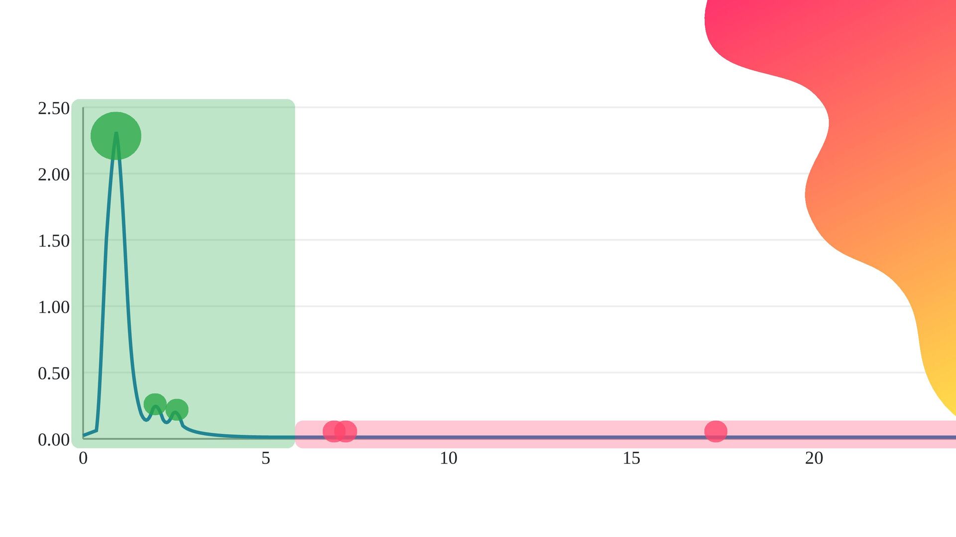
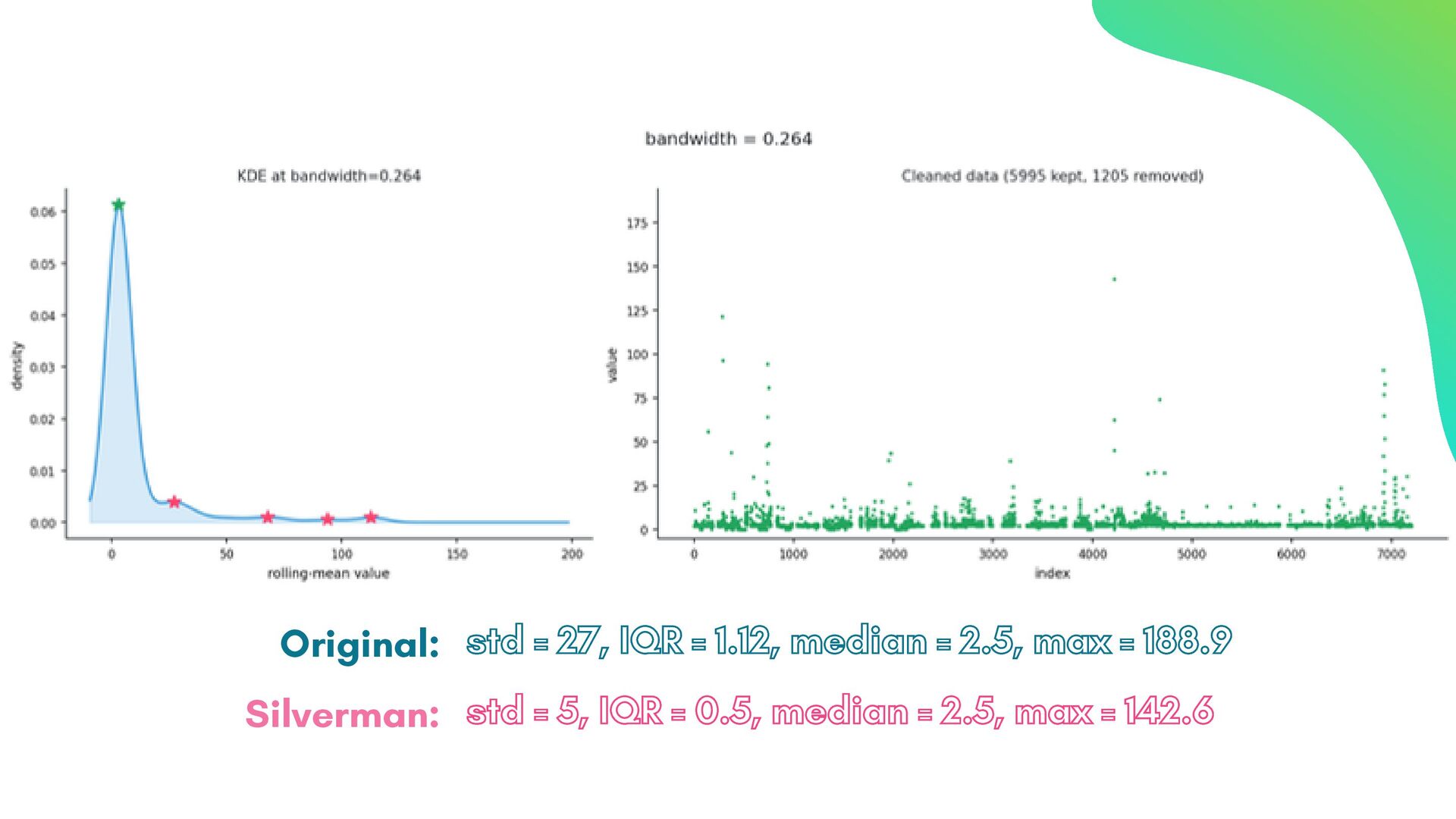
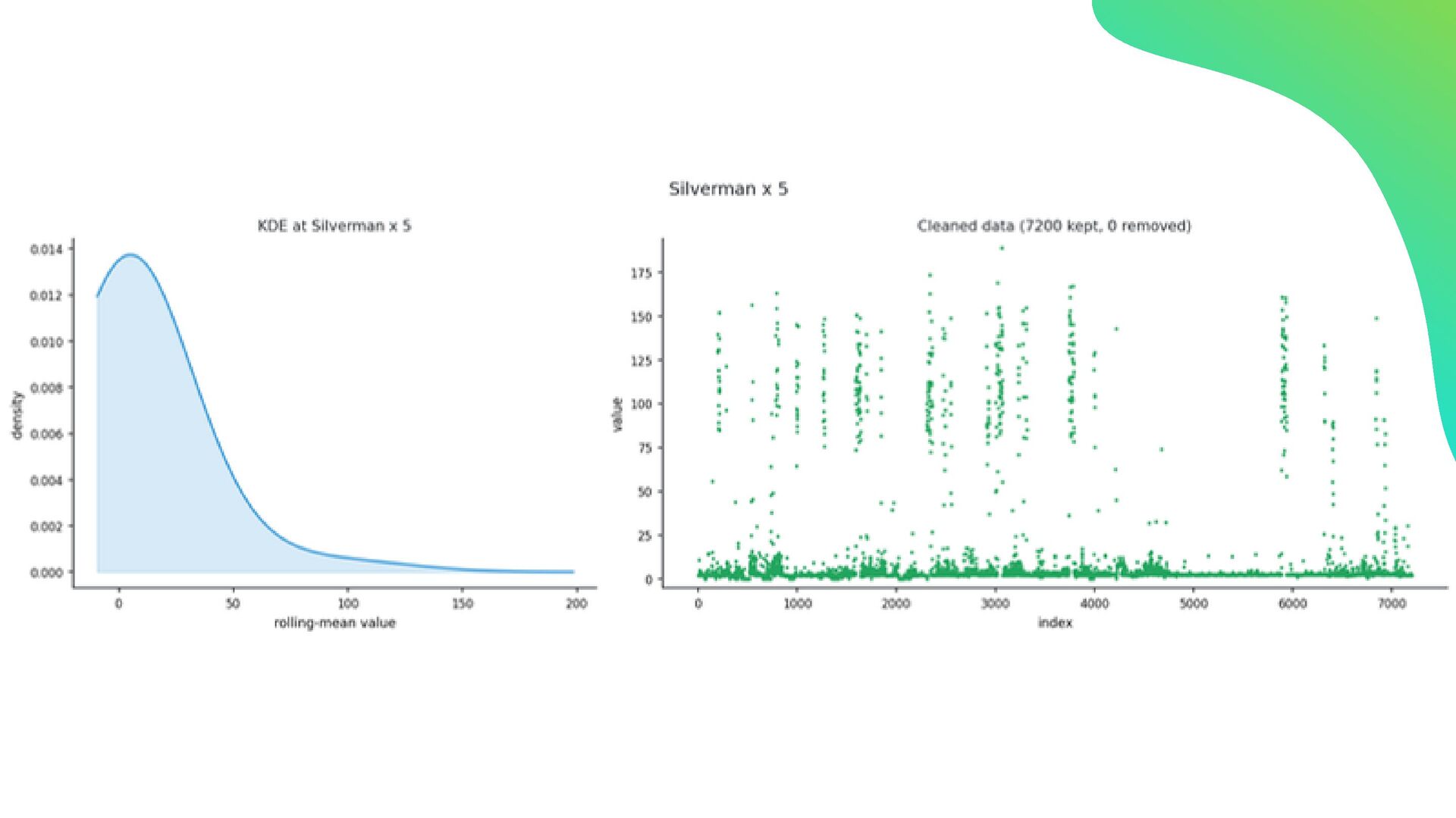
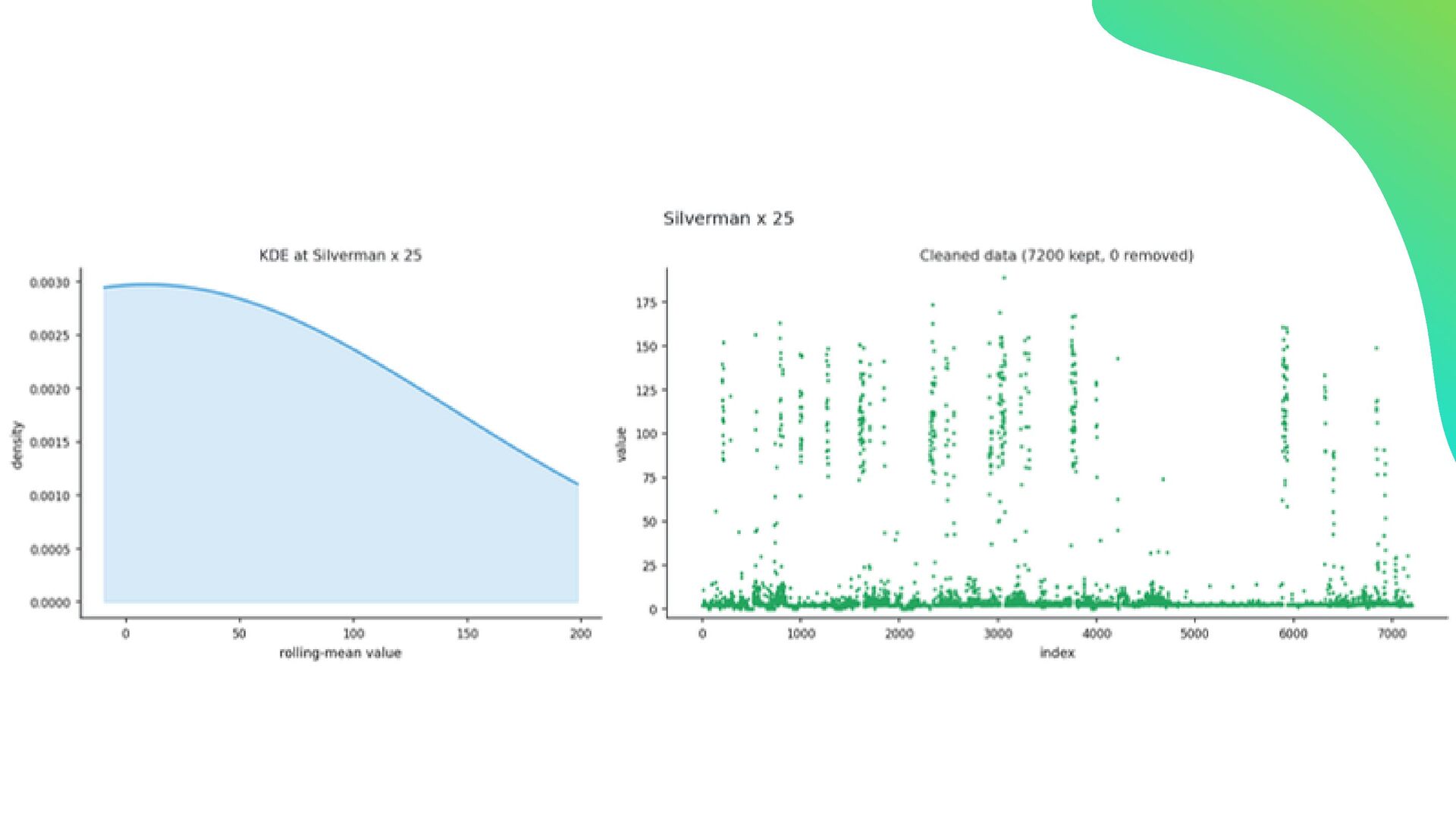
17. From Histogram to KDE 1. Histogram (6 bins) blocky bins 2. Each point gets a kernel each point = a bump (kernel) 3. Sum the kernels → KDE smooth curve main peak 2nd peak Time Series time 0 2 4 6 8 10 12 Histogram (6 bins) 0-2 2-4 4-6 6-8 8-10 10-12 KDE estimates the probability density KDE estimates the probability density
18. 0.00 0.50 1.00 1.50 2.00 2.50 0 5 10 15 20
19. D D F F G G Outliers A A B B C C E E
20. HEALTHY peak Inherits HEALTHY
21. 0.00 0.50 1.00 1.50 2.00 2.50 0 5 10 15 20
22. time_series.KDE ( kernel_shape, bandwidth ) KDE
23. Kernel Shapes Gaussian (most common) data point Triangle (Epanechnikov) data point Rectangle (uniform) data point time_series.KDE ( kernel_shape, bandwidth ) KDE
24. time_series.KDE ( kernel_shape, bandwidth ) KDE Small Bandwidth (bumpy, overfitting) details are overemphasized Large Bandwidth (smooth, underfitting) details are hidden
25. time_series.KDE ( kernel_shape, bandwidth ) KDE Silverman’s rule of thumb: Silverman’s rule of thumb: standard deviation interquartile range
26. Interquartile Range (IQR) Example: [2, 4, 5, 7, 8, 10, 12, 14, 15, 18, 20, 22] 2 4 5 7 8 10 12 14 15 18 20 22 left median = Q1 right median = Q3 median of all data 6th 7th
27. Interquartile Range (IQR) Example: [2, 4, 5, 7, 8, 10, 12, 14, 15, 18, 20, 22] 2 4 5 7 8 10 12 14 15 18 20 22 Q1 = 6.0 = median[2, 4, 5, 7, 8, 10] = (5+7) / 2 = 6 Q3 = 16.5 median[12, 14, 15, 18, 20, 22] = (15+18) / 2 = 16.5 IQR = Q3 - Q1 = 16.5 - 6.0 = 10.5 25% 50% 25%
28. Std vs IQR Scenario 1: Normal Data [1, 2, 3, 4, 5, 6, 7, 8, 9, 10] 1 5 10 std = 2.9 IQR = 5 → IQR/1.35 = 3.7 Similar! Both ~3 Scenario 2: One Outlier [1, 2, 3, 4, 5, 6, 7, 8, 9, 50] 1 9 50 std = 14.2 (wrecked!) IQR = 5 → IQR/1.35 = 3.7 IQR wins - ignores outlier Scenario 3: Mostly Same [0, 0, 0, 0, 0, 0, 0, 0, 1, 1] 0 (x8) 1 (x2) std = 0.4 IQR = 0 (all middle = 0) Std wins - sees the 1s
30. KDE KDE KDE × 5 (smoother curve) ÷ 3 (more bumpy curve) 3.8 × 5 = 19 19 ÷ 3 = 6.3 rule = 3.8
31. std = 27, IQR = 1.12, median = 2.5, max = 188.9 std = 27, IQR = 1.12, median = 2.5, max = 188.9
32. std = 27, IQR = 1.12, median = 2.5, max = 188.9 std = 27, IQR = 1.12, median = 2.5, max = 188.9 Original: std = 5, IQR = 0.5, median = 2.5, max = 142.6 std = 5, IQR = 0.5, median = 2.5, max = 142.6 Silverman:
35. std = 5, IQR = 0.5, median = 2.5, max = 142.6 std = 5, IQR = 0.5, median = 2.5, max = 142.6 Silverman: std = 4, IQR = 0.5, median = 2.5, max = 142.6 std = 4, IQR = 0.5, median = 2.5, max = 142.6 Silverman / 3:
36. std = 4.0, IQR = 0.5, median = 2.5, max = 142.6 std = 4.0, IQR = 0.5, median = 2.5, max = 142.6 Silverman / 3: std = 2.5, IQR = 0.4, median = 2.5, max = 73.9 std = 2.5, IQR = 0.4, median = 2.5, max = 73.9 Silverman / 9:
37. std = 0.12, IQR = 0, median = 0 std = 0.12, IQR = 0, median = 0
38. std = 0.12, IQR = 0 std = 0.12, IQR = 0 Original: std = 0.08, IQR = 0 std = 0.08, IQR = 0 Silverman: R E J E C T R E J E C T R E J E C T
39. 5XX response DB deadlock
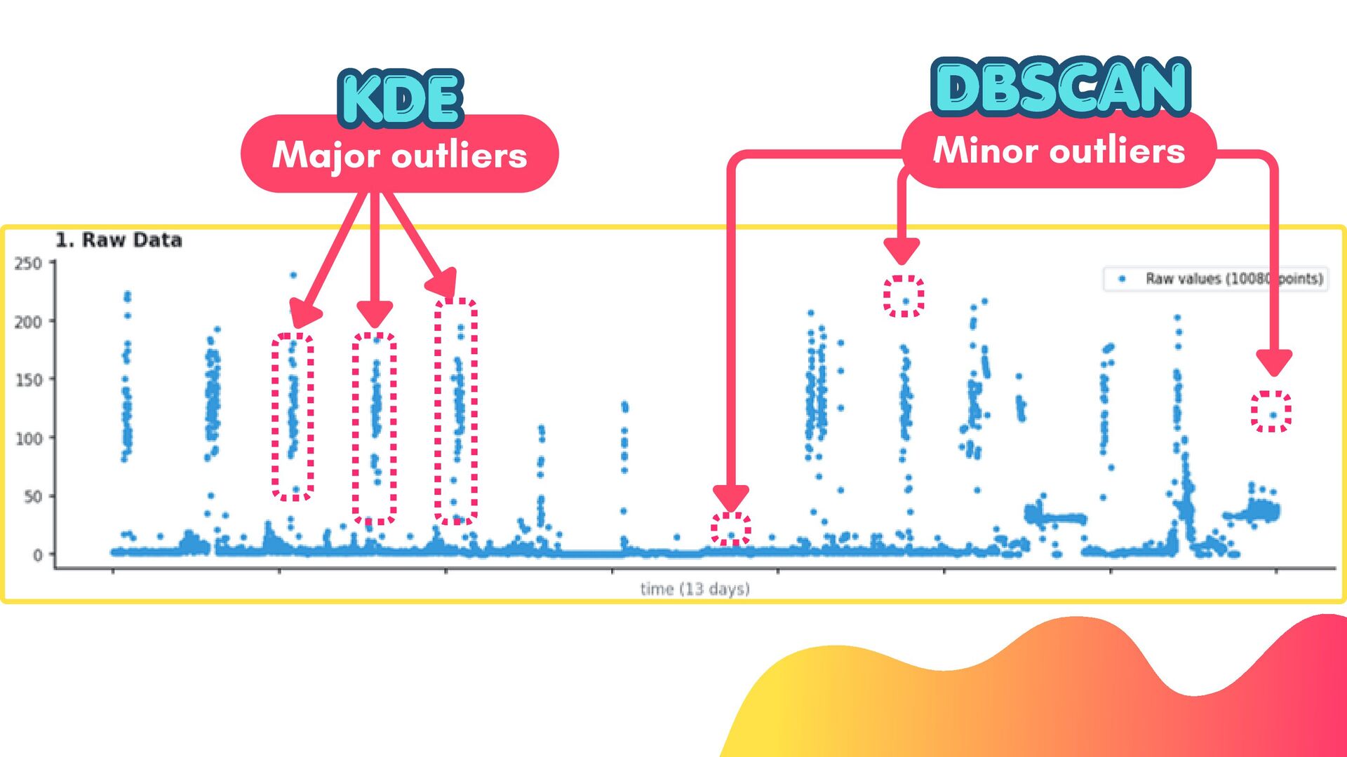
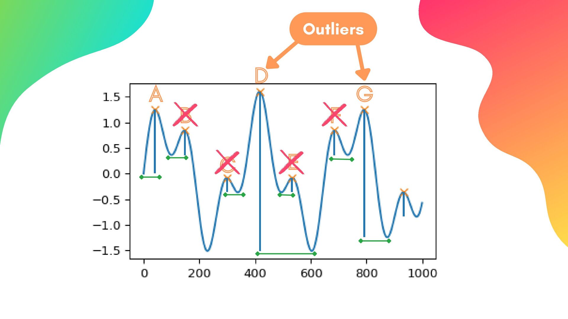
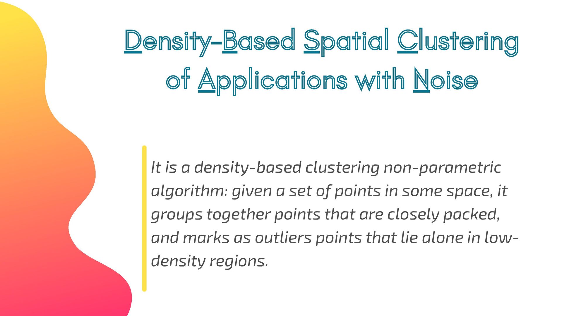
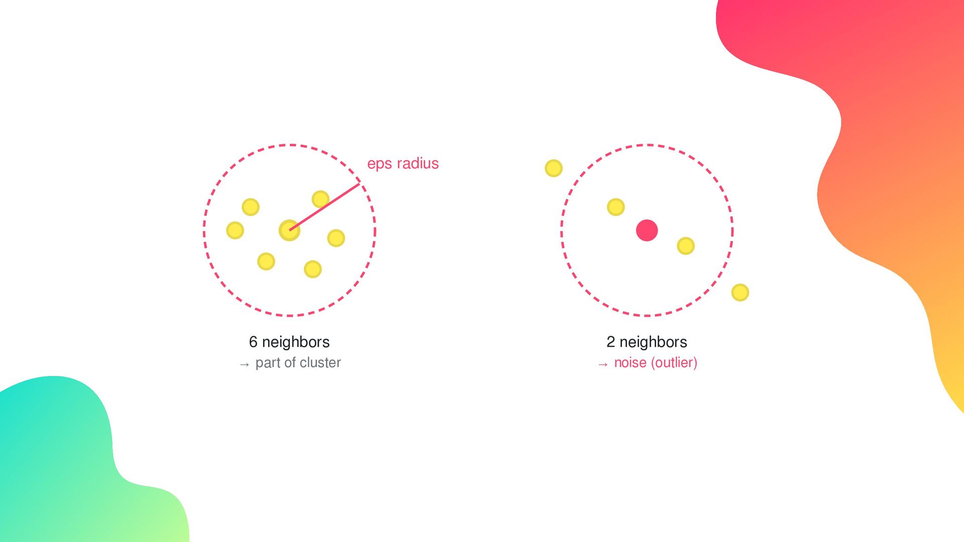
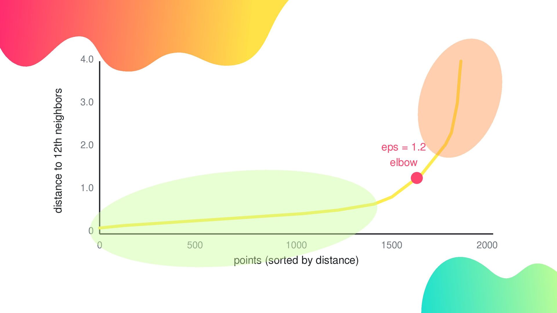
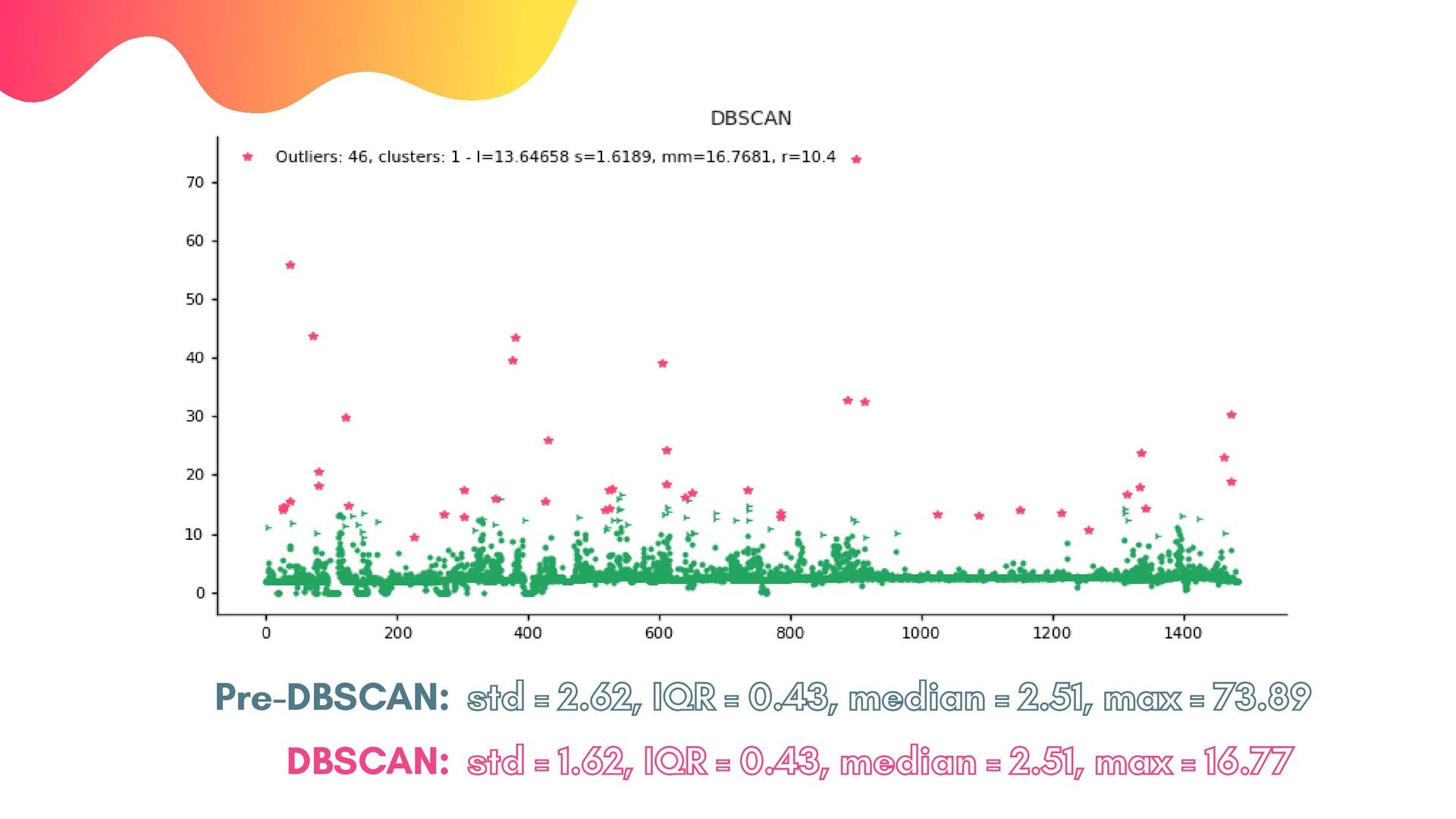
40. D D ensity- ensity- B B ased ased S S patial patial C C lustering lustering of of A A pplications with pplications with N N oise oise It is a density-based clustering non-parametric algorithm: given a set of points in some space, it groups together points that are closely packed, and marks as outliers points that lie alone in low- density regions.
41. Double Datetime 2D
42. 2D std / 10 std / 10 std / 10
43. eps radius 6 neighbors → part of cluster 2 neighbors → noise (outlier)
44. ε ε The Elbow Method
45. distance to 12th neighbors 0 1.0 2.0 3.0 4.0 points (sorted by distance) 0 500 1000 1500 2000 elbow eps = 1.2
46. std = 2.62, IQR = 0.43, median = 2.51, max = 73.89 std = 2.62, IQR = 0.43, median = 2.51, max = 73.89 Pre-DBSCAN:
47. epsilon = 6.87 epsilon = 6.87
48. std = 2.62, IQR = 0.43, median = 2.51, max = 73.89 std = 2.62, IQR = 0.43, median = 2.51, max = 73.89 Pre-DBSCAN: std = 1.62, IQR = 0.43, median = 2.51, max = 16.77 std = 1.62, IQR = 0.43, median = 2.51, max = 16.77 DBSCAN:
49. original epsilon = 6.87 original epsilon = 6.87 2nd epsilon = 34.12 2nd epsilon = 34.12
52. average ± 3σ average ± 3 σ ⇒ ⇒ 99.7% 99.7%
59. Link to sources Ines Panker | Jun 2026 Rate the Talk R ate the Talk Rate the Talk