Joint k-q space Compressed Sensing Diffusion MRI in ISMRM 2014

Joint k-q Space Compressed Sensing for Accelerated
Multi-Shell Acquisition and Reconstruction of the
diffusion signal and Ensemble Average Propagator

Transcript

1. Joint k-q Space Compressed Sensing for Accelerated Multi-Shell Acquisition and Reconstruction of the diffusion signal and Ensemble Average Propagator Jian Cheng, Dinggang Shen, Pew-Thian Yap May 14, 2014
2. Declaration
3. Outline 1 Motivation and Objective 2 6D-CS-dMRI 3 Experiments 4 Conclusion
4. Outline 1 Motivation and Objective 2 6D-CS-dMRI 3 Experiments 4 Conclusion
5. Reconstruction in 3D space Reconstruction problem: {S(x, qj )} → P(x, R) Fourier transform [Callaghan 1991] S(x, q) = S(x, 0) R∈R3 P(x, R)e−2πiqT RdR
6. Reconstruction in 3D space Reconstruction problem: {S(x, qj )} → P(x, R) Fourier transform [Callaghan 1991] S(x, q) = S(x, 0) R∈R3 P(x, R)e−2πiqT RdR Diffusion Tensor Imaging (DTI) [Basser 1994] : assumption is too strong to be correct Diffusion Spectrum Imaging (DSI) [Wedeen 2000, 2005] : assumption is too week to be practical
7. Compressed Sensing dMRI in 3D q-space Compressed Sensing (CS): reduce the number of samples, keep reconstruction quality. [Donoho 2006; Cand` es 2006]
8. Compressed Sensing dMRI in 3D q-space Compressed Sensing (CS): reduce the number of samples, keep reconstruction quality. [Donoho 2006; Cand` es 2006] CS-dMRI using 3D continuous sparse dictionary Simple Harmonic Oscillator based Reconstruction and Estimation (SHORE) [¨ Ozarslan 2009, 2013] Spherical Polar Fourier Imaging (SPFI) [Assemlal 2009, Cheng 2010, 2011, 2013], Significant reduction of scanning time?
9. Outline 1 Motivation and Objective 2 6D-CS-dMRI 3 Experiments 4 Conclusion
10. CS-dMRI in joint 6D k-q space (6D-CS-dMRI) Reconstruction problem: {S(km , qj )} → P(x , R) S(k, q) = x∈R3 S(x, 0) R∈R3 P(x, R)e−2πiqT RdRe−2πixT kdx Joint sampling in both k-space and q-space. [Mani 2012, 2014; Awate 2013] total scanning time reduction: R = RkRq.
11. A naive way of 6D-CS-dMRI Two steps: {S(km , qj)} → {S(x , qj )} → P(x, R) Pros: Fast, easy to be implemented: volume by volume [Lustig 2007], voxel by voxel [Cheng 2013]
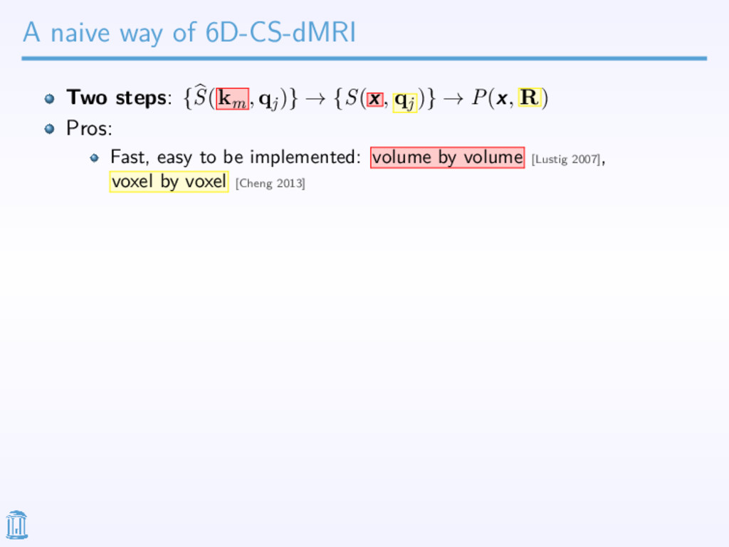
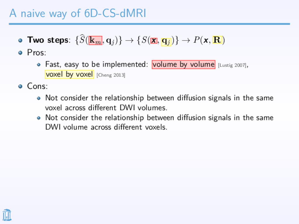
12. A naive way of 6D-CS-dMRI Two steps: {S(km , qj)} → {S(x , qj )} → P(x, R) Pros: Fast, easy to be implemented: volume by volume [Lustig 2007], voxel by voxel [Cheng 2013] Cons: Not consider the relationship between diffusion signals in the same voxel across different DWI volumes. Not consider the relationship between diffusion signals in the same DWI volume across different voxels.
13. 6D-CS-dMRI using joint optimization Reconstruction problem: {S(km , qj )} → P(x , R) min {ci },{sv} Nq v=1 Fp sv − sv 2 2 + λ1 TV(sv ) + λ2 Φsv 1 + λ3 Ns i=1 ci 1 s.t. Mci = Re{si} ∀i, Nq: number of volumes, v = 1, 2, . . . , Nq Ns: number of voxels, i = 1, 2, . . . , Ns sv: measurements in k-space for v-th volume sv: DWI signal vector in v-th volume si: DWI signal vector in i-th voxel Fp: partial Fourier transform Φ: wavelet basis ci: coefficient vector in i-th voxel M: basis matrix with basis elements in its columns λ1, λ2 , λ3 : regularization parameters Re: real part
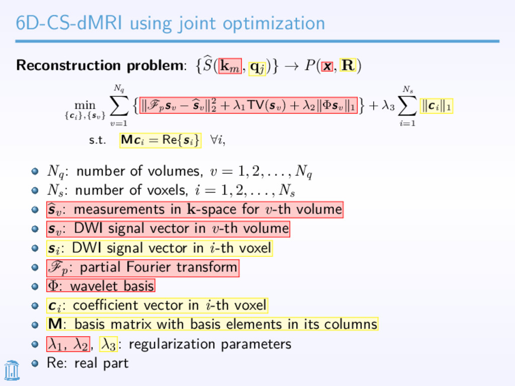
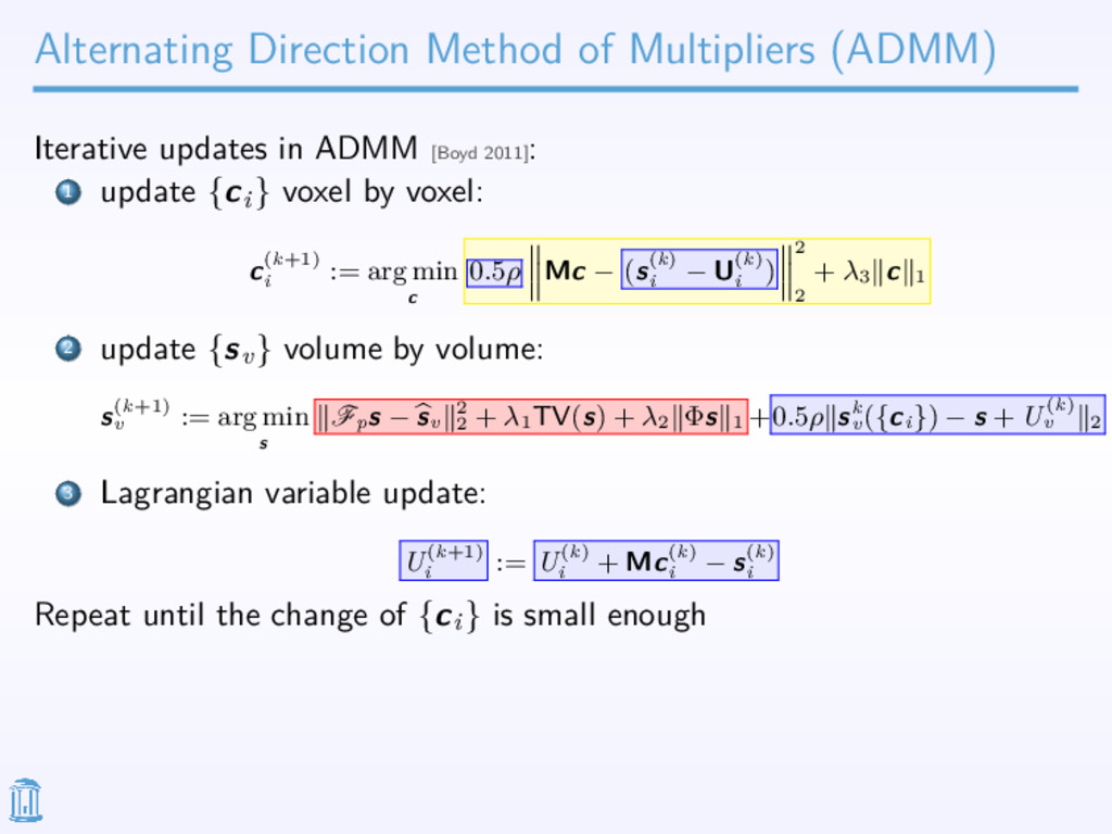
14. Alternating Direction Method of Multipliers (ADMM) Iterative updates in ADMM [Boyd 2011] : 1 update {ci} voxel by voxel: c(k+1) i := arg min c 0.5ρ Mc − (s(k) i − U(k) i ) 2 2 + λ3 c 1 2 update {sv} volume by volume: s(k+1) v := arg min s Fp s − sv 2 2 + λ1 TV(s) + λ2 Φs 1 +0.5ρ sk v ({ci}) − s + U(k) v 2 3 Lagrangian variable update: U(k+1) i := U(k) i + Mc(k) i − s(k) i Repeat until the change of {ci} is small enough
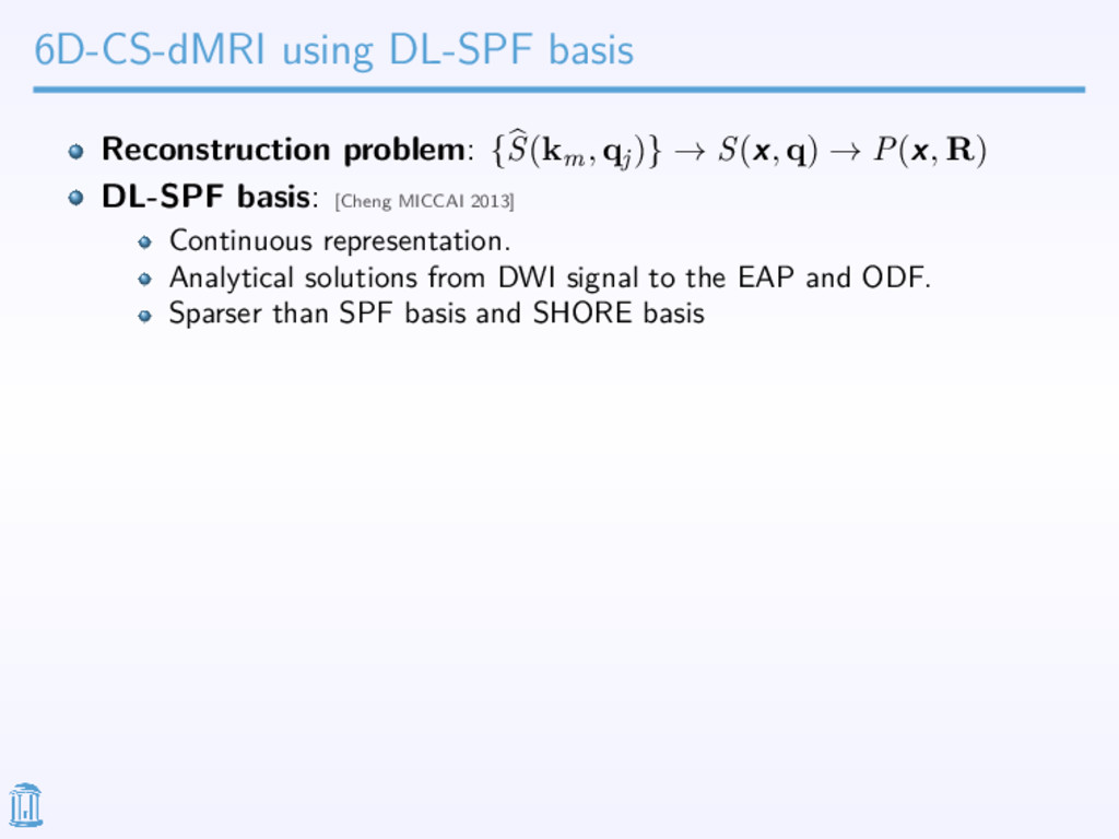
15. 6D-CS-dMRI using DL-SPF basis Reconstruction problem: {S(km, qj)} → S(x, q) → P(x, R) DL-SPF basis: [Cheng MICCAI 2013] Continuous representation. Analytical solutions from DWI signal to the EAP and ODF. Sparser than SPF basis and SHORE basis
16. Outline 1 Motivation and Objective 2 6D-CS-dMRI 3 Experiments 4 Conclusion
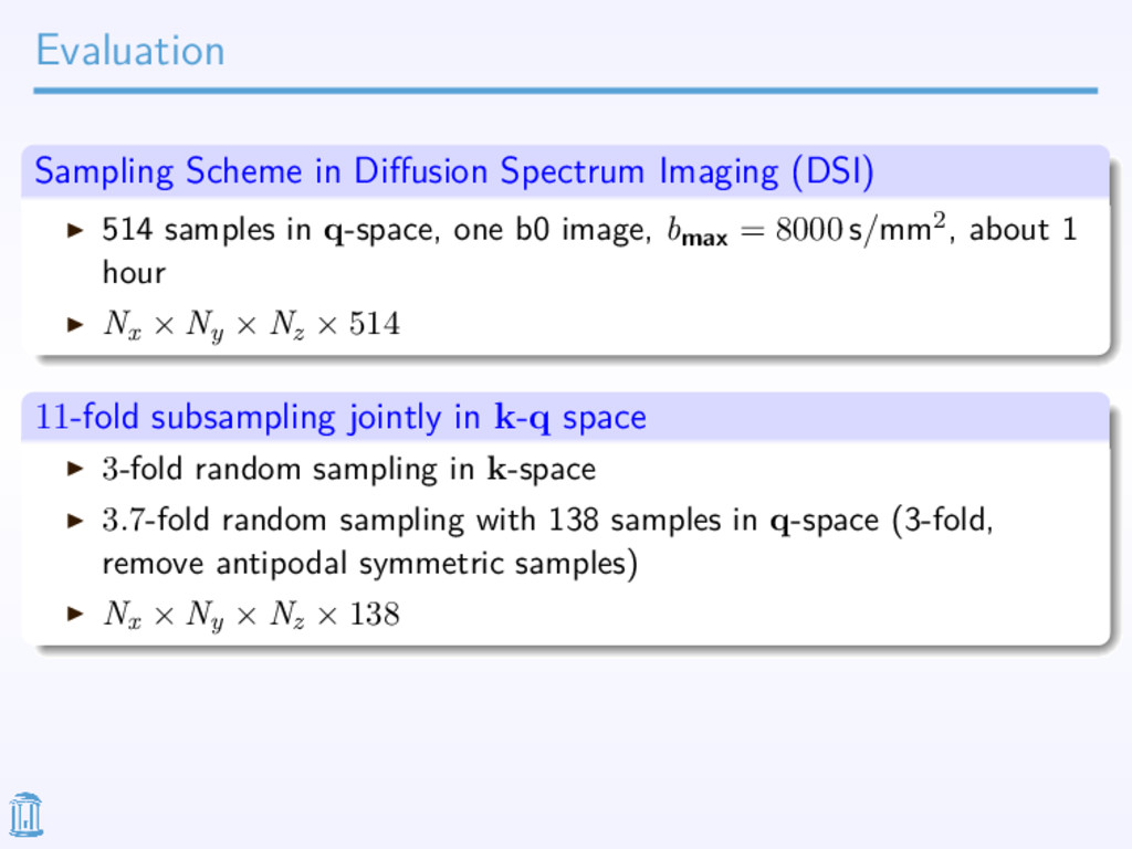
17. Evaluation Sampling Scheme in Diffusion Spectrum Imaging (DSI) I 514 samples in q-space, one b0 image, bmax = 8000 s/mm2, about 1 hour I Nx × Ny × Nz × 514 11-fold subsampling jointly in k-q space I 3-fold random sampling in k-space I 3.7-fold random sampling with 138 samples in q-space (3-fold, remove antipodal symmetric samples) I Nx × Ny × Nz × 138
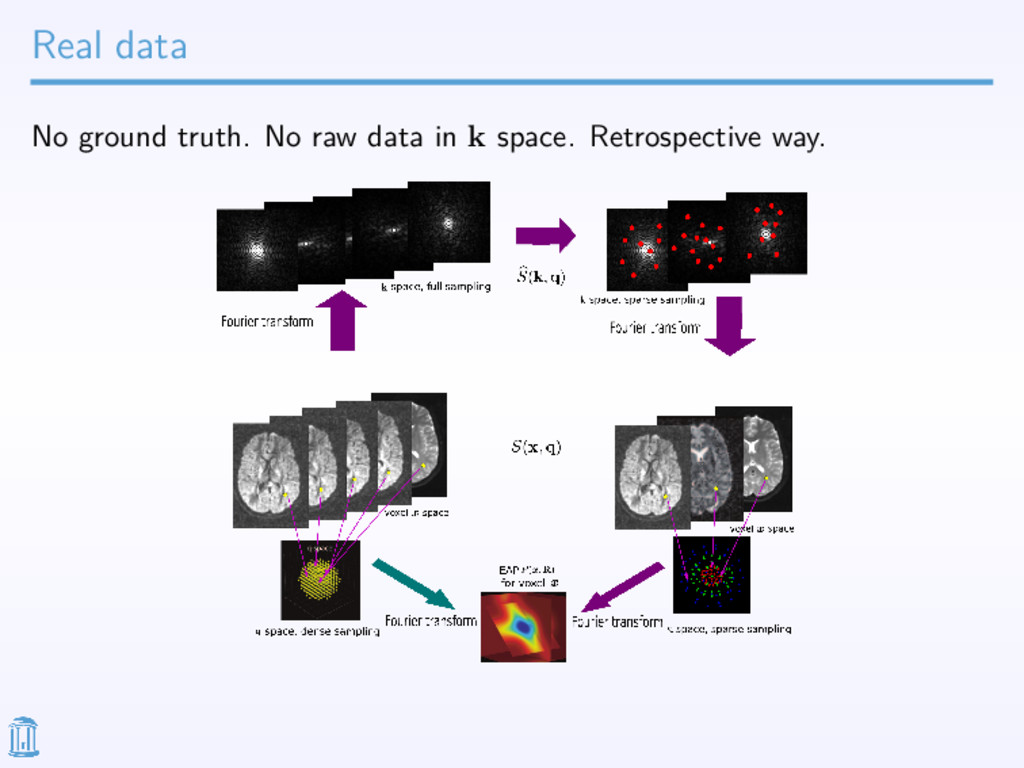
18. Evaluation Correctness and Consistency I Synthetic data: test correctness by comparing the reconstruction result using 11-fold subsampling with the ground truth I Real data test consistency by comparing the reconstruction result using 11-fold subsampling with the reconstruction result using DSI sampling Root Mean Square Error (RMSE) I In each voxel, RMSE is defined on 514 DWI samples in DSI scheme. I In a field, we calculate the mean RMSE.
19. Synthetic Data without noise EAP profiles with radius 15µm, 20 × 20 × 1 × 514 6D-CS-dMRI, no noise Naive, no noise Mean RMSE: 3.20% Mean RMSE: 7.97%
20. Synthetic Data with noise Add Gaussian noise in measurements in k-space. 6D-CS-dMRI, SNR=25 Naive, SNR=25 Mean RMSE: 7.60% Mean RMSE: 12.76%
21. Real data No ground truth. No raw data in k space. Retrospective way.
22. Real data From HCP project 6D-CS-dMRI, no noise Naive, no noise Mean RMSE: 5.15% Mean RMSE: 7.78%
23. Real data Add Gaussian noise in measurements in k-space. 6D-CS-dMRI, SNR=25 Naive, SNR=25 Mean RMSE: 8.83% Mean RMSE: 14.06%
24. Outline 1 Motivation and Objective 2 6D-CS-dMRI 3 Experiments 4 Conclusion
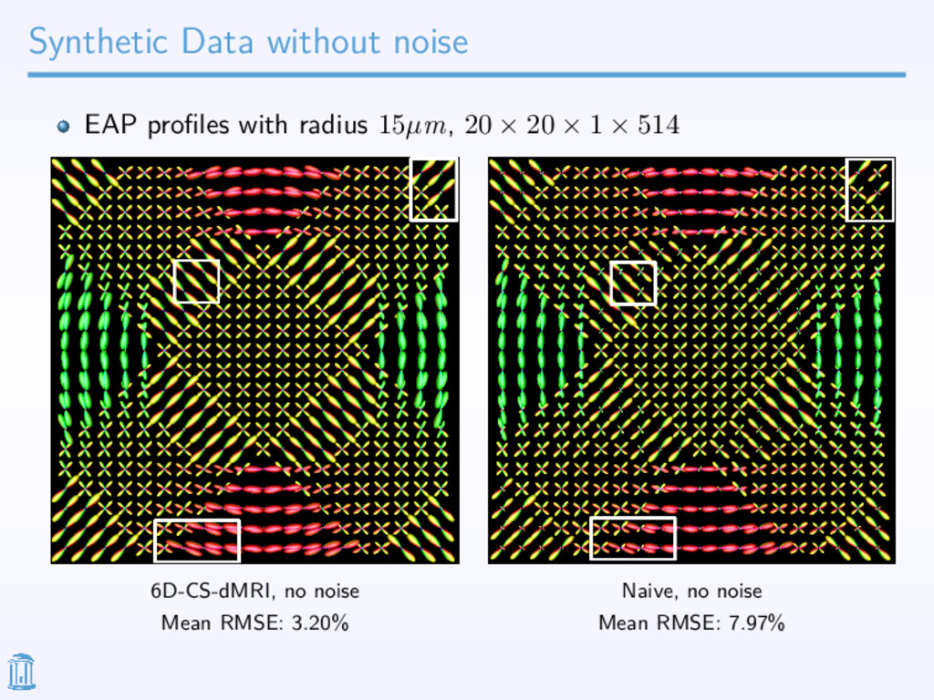
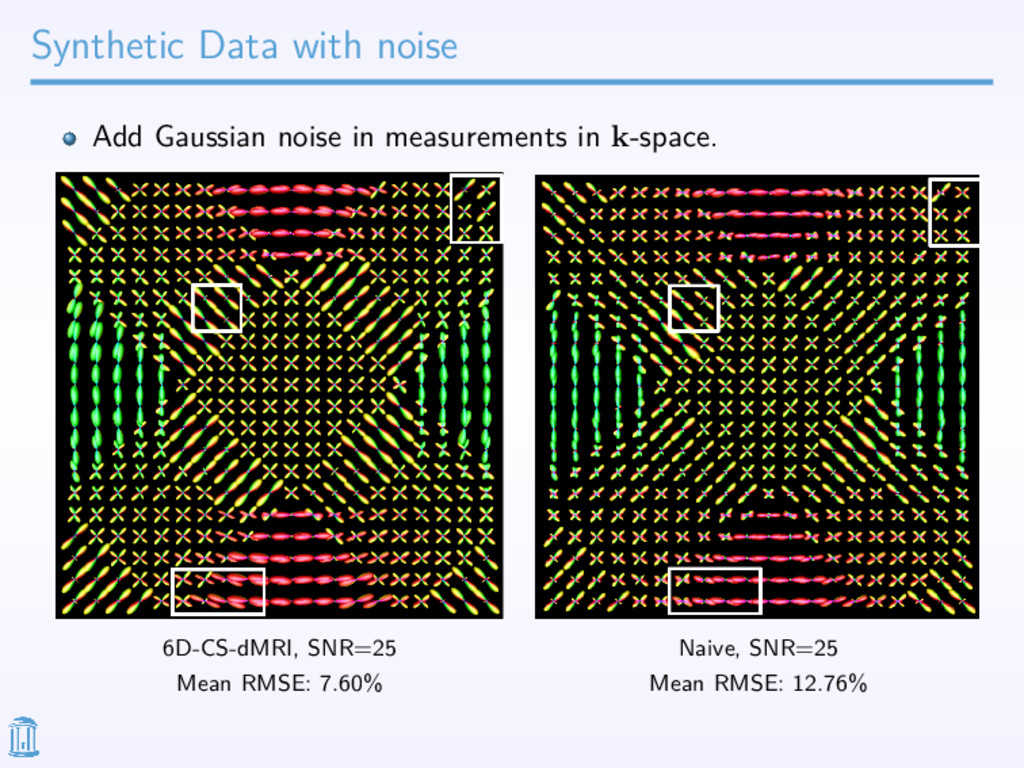
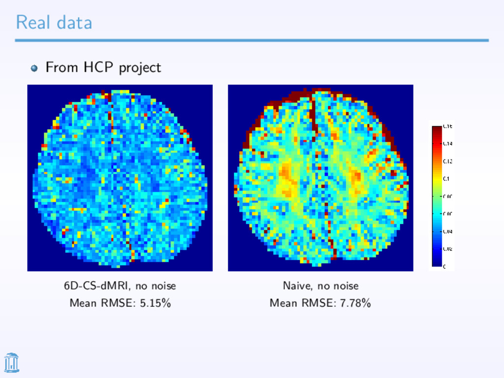
25. Conclusion and Prospective Conclusion: 6D-CS-dMRI performs CS reconstruction of diffusion signal and propagator in joint k-q space. 6D-CS-dMRI has lower RMSE and more robust to noise than its naive way. 6D-CS-dMRI achieves RMSE about 5% by using 11-fold subsampling in k-q space. Future work: Acquire raw complex data in k-space. Sampling scheme in q-space: a subset of DSI scheme → multi-shell uniform sampling scheme. (poster id: 2558. Wednesday, 4pm-6pm. MICCAI 2014) Efficient implementation: parallel in different volumes and different voxels
26. Thank you!