Entangled Quantum walk

Quantum walk on quantum games.

Transcript

1. Entangled Quantum Walks Jishnu Rajendran Supervisor:Colin Benjamin National Institute of Science Education and Research jishnu.r@niser.ac.in November 25,2016 Jishnu Rajendran (NISER) Quantum Walk November 25,2016 1 / 39
2. Overview 1 Introduction to Random Walk Classical Random walk Basic properties of a classical walk Quantum walk Basic introduction to Quantum walk Defining Quantum Walk Probability distribution of a QW Symmetric Discrete Time quantum walk Results to the Symmetric Discrete Time quantum walk 2 Parrondo’s game 3 Parrondo’s game using Quantum Walk Construction of the game Analyzing the results 4 Entangled Quantum walk Definitions and processes involved Results 5 Entangled Parrondo’s quantum walk 6 References Jishnu Rajendran (NISER) Quantum Walk November 25,2016 2 / 39
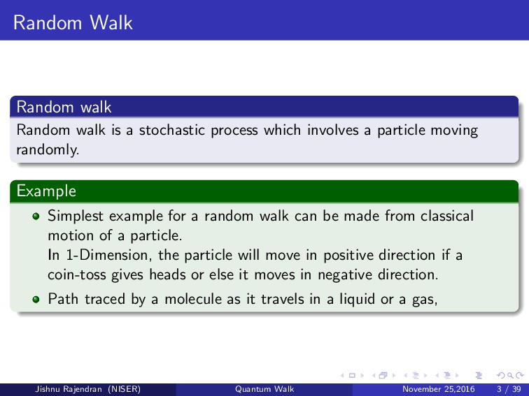
3. Random Walk Random walk Random walk is a stochastic process which involves a particle moving randomly. Example Simplest example for a random walk can be made from classical motion of a particle. In 1-Dimension, the particle will move in positive direction if a coin-toss gives heads or else it moves in negative direction. Path traced by a molecule as it travels in a liquid or a gas, Jishnu Rajendran (NISER) Quantum Walk November 25,2016 3 / 39
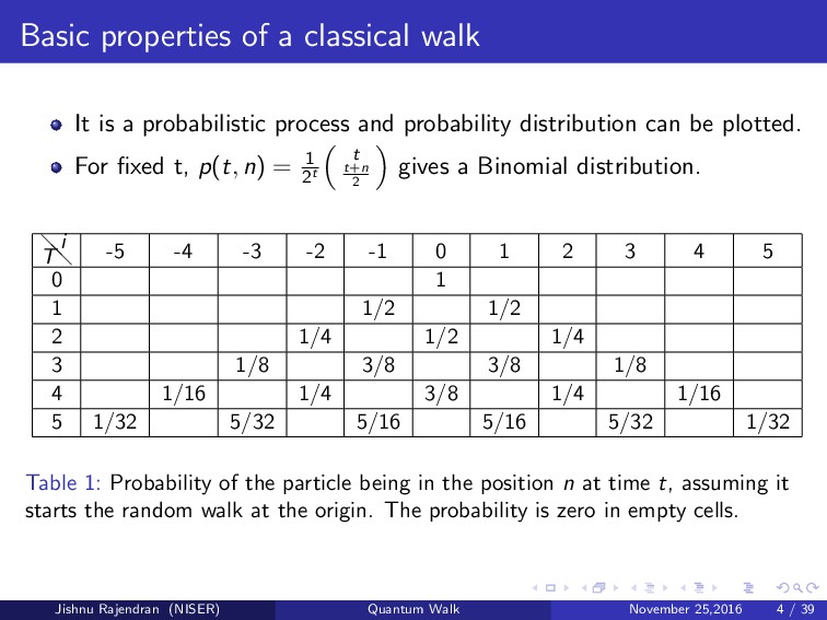
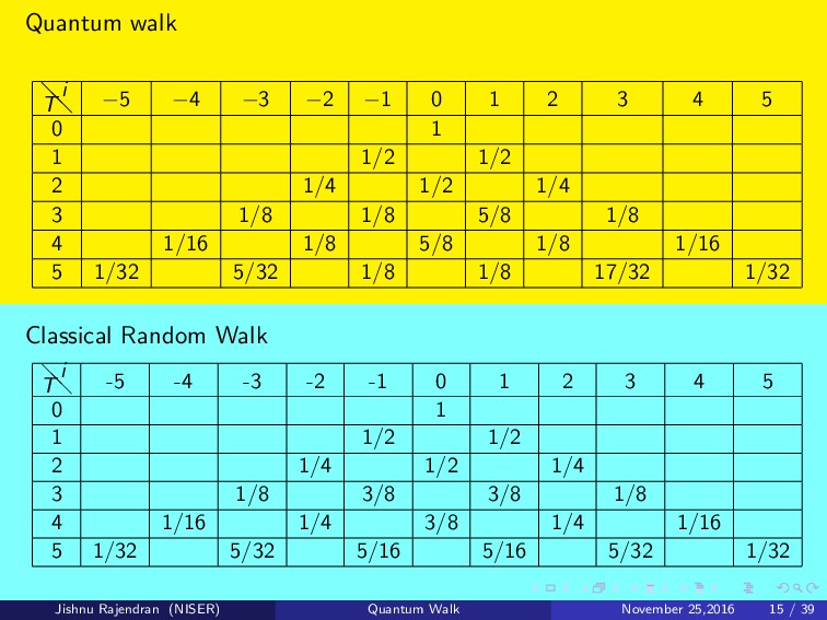
4. Basic properties of a classical walk It is a probabilistic process and probability distribution can be plotted. For fixed t, p(t, n) = 1 2t t t+n 2 gives a Binomial distribution. @ @ T i -5 -4 -3 -2 -1 0 1 2 3 4 5 0 1 1 1/2 1/2 2 1/4 1/2 1/4 3 1/8 3/8 3/8 1/8 4 1/16 1/4 3/8 1/4 1/16 5 1/32 5/32 5/16 5/16 5/32 1/32 Table 1: Probability of the particle being in the position n at time t, assuming it starts the random walk at the origin. The probability is zero in empty cells. Jishnu Rajendran (NISER) Quantum Walk November 25,2016 4 / 39
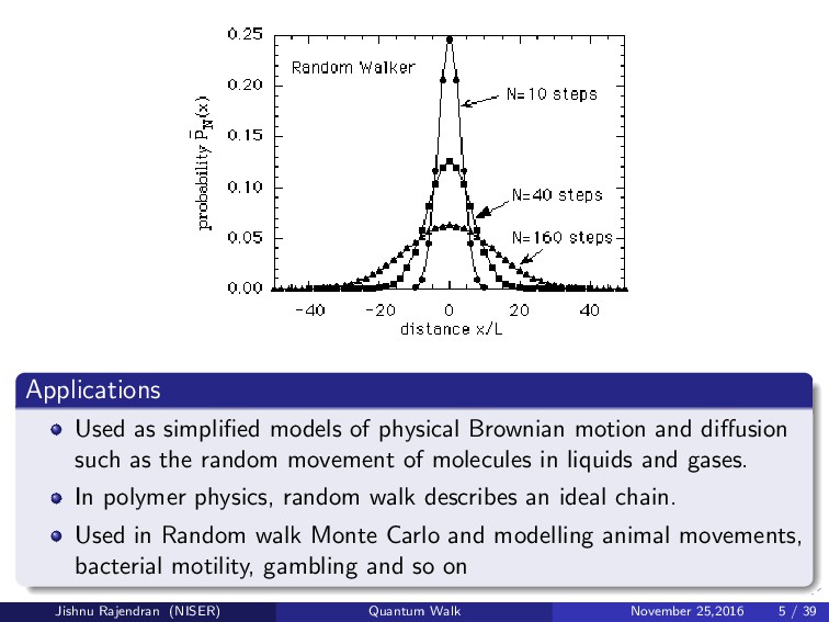
5. Applications Used as simplified models of physical Brownian motion and diffusion such as the random movement of molecules in liquids and gases. In polymer physics, random walk describes an ideal chain. Used in Random walk Monte Carlo and modelling animal movements, bacterial motility, gambling and so on Jishnu Rajendran (NISER) Quantum Walk November 25,2016 5 / 39
6. Quantum walk Motivation Quantum walks are motivated by the widespread use of classical random walks in wide range of problems. Quantum walks exhibits very different behavior from classical random walks,which will discussed. Two types of quantum walk There are two types of quantum walk 1. Discrete Time Quantum Walk. 2. Continuous Time Quantum Walk Our main focus will be on DTQW Jishnu Rajendran (NISER) Quantum Walk November 25,2016 6 / 39
7. Difference between Classical and quantum walk Jishnu Rajendran (NISER) Quantum Walk November 25,2016 7 / 39
8. Basic introduction to Quantum walk By the process of quantization, each measurable parameter in a physical system is associated with a quantum mechanical operator acting on a Hilbert space. The state of the quantum system is described by a vector in the Hilbert space and the evolution of the system is governed by a unitary operation. Even though the evolution of the system is completely deterministic,the process of measurement generates the probability distribution. Jishnu Rajendran (NISER) Quantum Walk November 25,2016 8 / 39
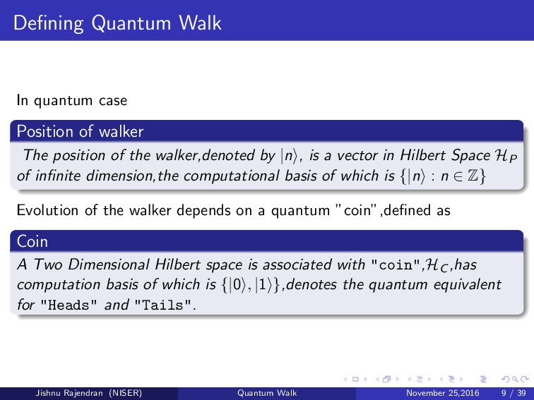
9. Defining Quantum Walk In quantum case Position of walker The position of the walker,denoted by |n , is a vector in Hilbert Space HP of infinite dimension,the computational basis of which is {|n : n ∈ Z} Evolution of the walker depends on a quantum ”coin”,defined as Coin A Two Dimensional Hilbert space is associated with "coin",HC ,has computation basis of which is {|0 , |1 },denotes the quantum equivalent for "Heads" and "Tails". Jishnu Rajendran (NISER) Quantum Walk November 25,2016 9 / 39
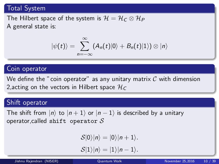
10. Total System The Hilbert space of the system is H = HC ⊗ HP A general state is: |ψ(t) = ∞ n=−∞ (An(t)|0 + Bn(t)|1 ) ⊗ |n Coin operator We define the ”coin operator” as any unitary matrix C with dimension 2,acting on the vectors in Hilbert space HC Shift operator The shift from |n to |n + 1 or |n − 1 is described by a unitary operator,called shift operator S S|0 |n = |0 |n + 1 . S|1 |n = |1 |n − 1 . Jishnu Rajendran (NISER) Quantum Walk November 25,2016 10 / 39
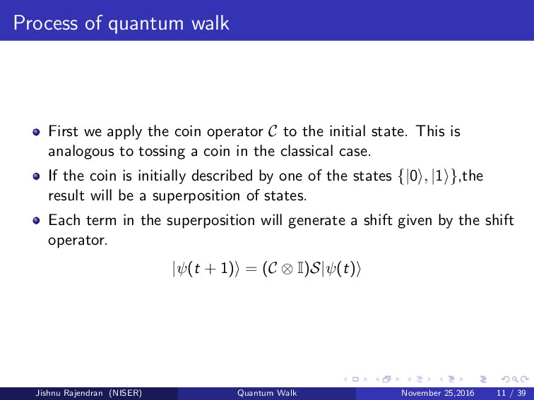
11. Process of quantum walk First we apply the coin operator C to the initial state. This is analogous to tossing a coin in the classical case. If the coin is initially described by one of the states {|0 , |1 },the result will be a superposition of states. Each term in the superposition will generate a shift given by the shift operator. |ψ(t + 1) = (C ⊗ I)S|ψ(t) Jishnu Rajendran (NISER) Quantum Walk November 25,2016 11 / 39
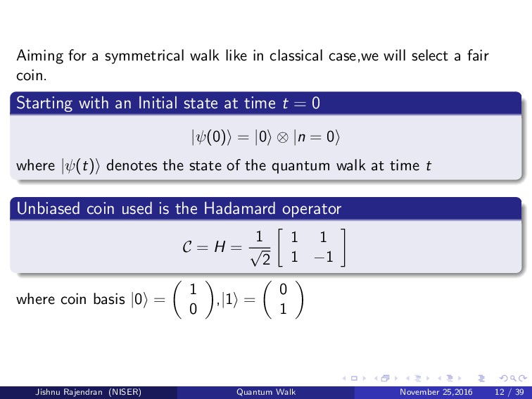
12. Aiming for a symmetrical walk like in classical case,we will select a fair coin. Starting with an Initial state at time t = 0 |ψ(0) = |0 ⊗ |n = 0 where |ψ(t) denotes the state of the quantum walk at time t Unbiased coin used is the Hadamard operator C = H = 1 √ 2 1 1 1 −1 where coin basis |0 = 1 0 ,|1 = 0 1 Jishnu Rajendran (NISER) Quantum Walk November 25,2016 12 / 39
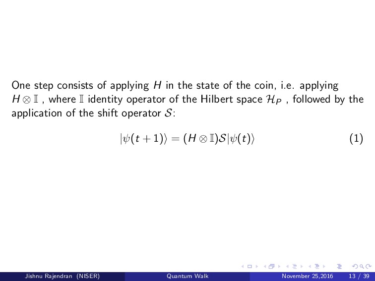
13. One step consists of applying H in the state of the coin, i.e. applying H ⊗ I , where I identity operator of the Hilbert space HP , followed by the application of the shift operator S: |ψ(t + 1) = (H ⊗ I)S|ψ(t) (1) Jishnu Rajendran (NISER) Quantum Walk November 25,2016 13 / 39
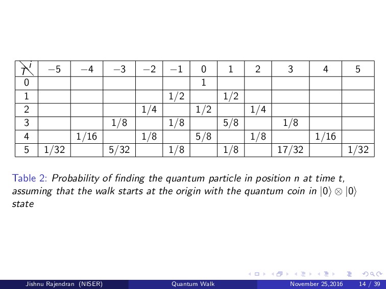
14. @ @ T i −5 −4 −3 −2 −1 0 1 2 3 4 5 0 1 1 1/2 1/2 2 1/4 1/2 1/4 3 1/8 1/8 5/8 1/8 4 1/16 1/8 5/8 1/8 1/16 5 1/32 5/32 1/8 1/8 17/32 1/32 Table 2: Probability of finding the quantum particle in position n at time t, assuming that the walk starts at the origin with the quantum coin in |0 ⊗ |0 state Jishnu Rajendran (NISER) Quantum Walk November 25,2016 14 / 39
15. Quantum walk @ @ T i −5 −4 −3 −2 −1 0 1 2 3 4 5 0 1 1 1/2 1/2 2 1/4 1/2 1/4 3 1/8 1/8 5/8 1/8 4 1/16 1/8 5/8 1/8 1/16 5 1/32 5/32 1/8 1/8 17/32 1/32 Classical Random Walk @ @ T i -5 -4 -3 -2 -1 0 1 2 3 4 5 0 1 1 1/2 1/2 2 1/4 1/2 1/4 3 1/8 3/8 3/8 1/8 4 1/16 1/4 3/8 1/4 1/16 5 1/32 5/32 5/16 5/16 5/32 1/32 Jishnu Rajendran (NISER) Quantum Walk November 25,2016 15 / 39
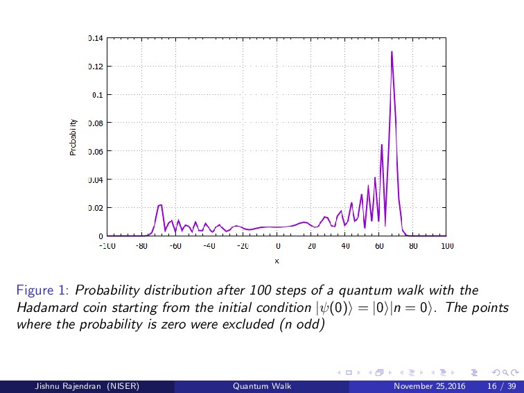
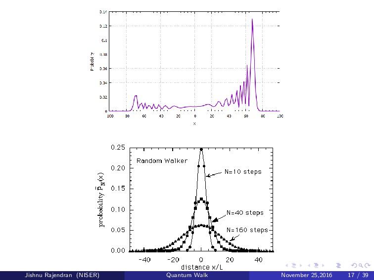
16. Figure 1: Probability distribution after 100 steps of a quantum walk with the Hadamard coin starting from the initial condition |ψ(0) = |0 |n = 0 . The points where the probability is zero were excluded (n odd) Jishnu Rajendran (NISER) Quantum Walk November 25,2016 16 / 39
17. Jishnu Rajendran (NISER) Quantum Walk November 25,2016 17 / 39
18. Reason behind the asymmetry The Hadamard coin introduces a negative sign when applied to state |1 . This means there are more cancellations of terms with coin state equals |1 than of terms with coin state equals |0 . Since the coin state |0 induces movement to right and |1 to left, the final effect is the asymmetry with large probabilities on the right. Similarly if the initial state is |ψ(0) = −|1 |n = 0 we will get a probability distribution asymmetric towards left side. Jishnu Rajendran (NISER) Quantum Walk November 25,2016 18 / 39
19. Symmetric Discrete Time quantum walk To obtain a symmetric distribution we need to take care of the cancellations and which can be achieved by taking an initial condition |ψ(0) = |0 + i|1 √ 2 |n = 0 Jishnu Rajendran (NISER) Quantum Walk November 25,2016 19 / 39
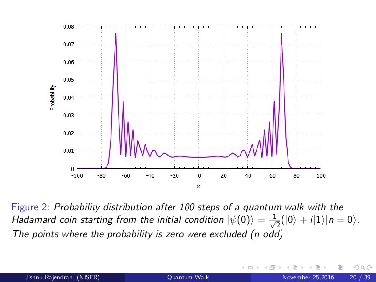
20. Figure 2: Probability distribution after 100 steps of a quantum walk with the Hadamard coin starting from the initial condition |ψ(0) = 1 √ 2 (|0 + i|1 |n = 0 . The points where the probability is zero were excluded (n odd) Jishnu Rajendran (NISER) Quantum Walk November 25,2016 20 / 39
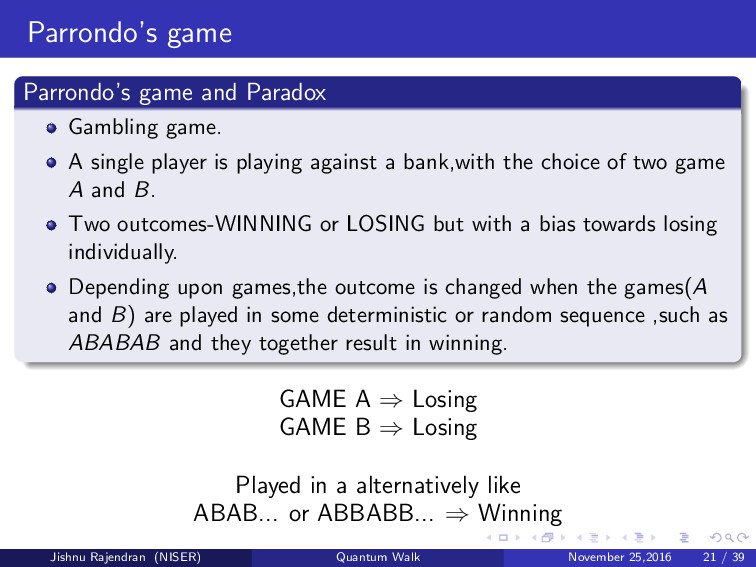
21. Parrondo’s game Parrondo’s game and Paradox Gambling game. A single player is playing against a bank,with the choice of two game A and B. Two outcomes-WINNING or LOSING but with a bias towards losing individually. Depending upon games,the outcome is changed when the games(A and B) are played in some deterministic or random sequence ,such as ABABAB and they together result in winning. GAME A ⇒ Losing GAME B ⇒ Losing Played in a alternatively like ABAB... or ABBABB... ⇒ Winning Jishnu Rajendran (NISER) Quantum Walk November 25,2016 21 / 39
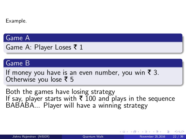
22. Example. Game A Game A: Player Loses | 1 Game B If money you have is an even number, you win | 3. Otherwise you lose | 5 Both the games have losing strategy If say, player starts with | 100 and plays in the sequence BABABA... Player will have a winning strategy Jishnu Rajendran (NISER) Quantum Walk November 25,2016 22 / 39
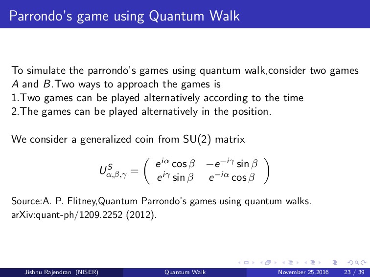
23. Parrondo’s game using Quantum Walk To simulate the parrondo’s games using quantum walk,consider two games A and B.Two ways to approach the games is 1.Two games can be played alternatively according to the time 2.The games can be played alternatively in the position. We consider a generalized coin from SU(2) matrix US α,β,γ = eiα cos β −e−iγ sin β eiγ sin β e−iα cos β Source:A. P. Flitney,Quantum Parrondo’s games using quantum walks. arXiv:quant-ph/1209.2252 (2012). Jishnu Rajendran (NISER) Quantum Walk November 25,2016 23 / 39
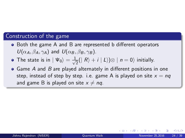
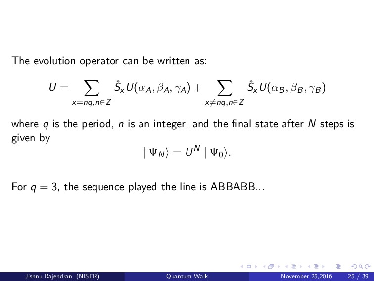
24. Construction of the game Both the game A and B are represented b different operators U(αA, βA, γA) and U(αB, βB, γB). The state is in | Ψ0 = 1 √ 2 (| R + i | L )⊗ | n = 0 initially. Game A and B are played alternately in different positions in one step, instead of step by step. i.e. game A is played on site x = nq and game B is played on site x = nq. Jishnu Rajendran (NISER) Quantum Walk November 25,2016 24 / 39
25. The evolution operator can be written as: U = x=nq,n∈Z ˆ Sx U(αA, βA, γA) + x=nq,n∈Z ˆ Sx U(αB, βB, γB) where q is the period, n is an integer, and the final state after N steps is given by | ΨN = UN | Ψ0 . For q = 3, the sequence played the line is ABBABB... Jishnu Rajendran (NISER) Quantum Walk November 25,2016 25 / 39
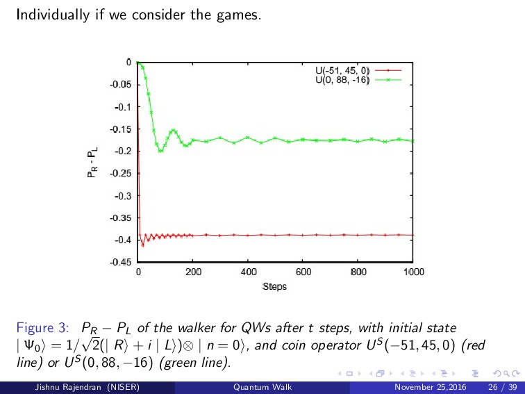
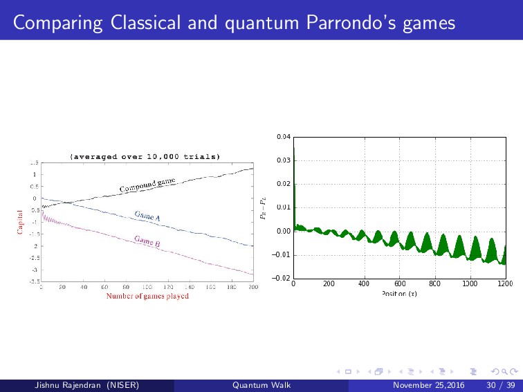
26. Individually if we consider the games. Figure 3: PR − PL of the walker for QWs after t steps, with initial state | Ψ0 = 1/ √ 2(| R + i | L )⊗ | n = 0 , and coin operator US (−51, 45, 0) (red line) or US (0, 88, −16) (green line). Jishnu Rajendran (NISER) Quantum Walk November 25,2016 26 / 39
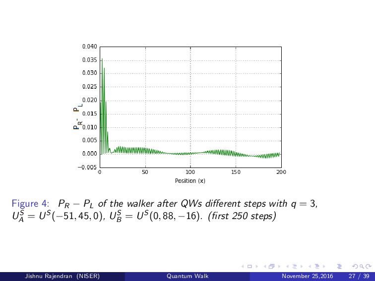
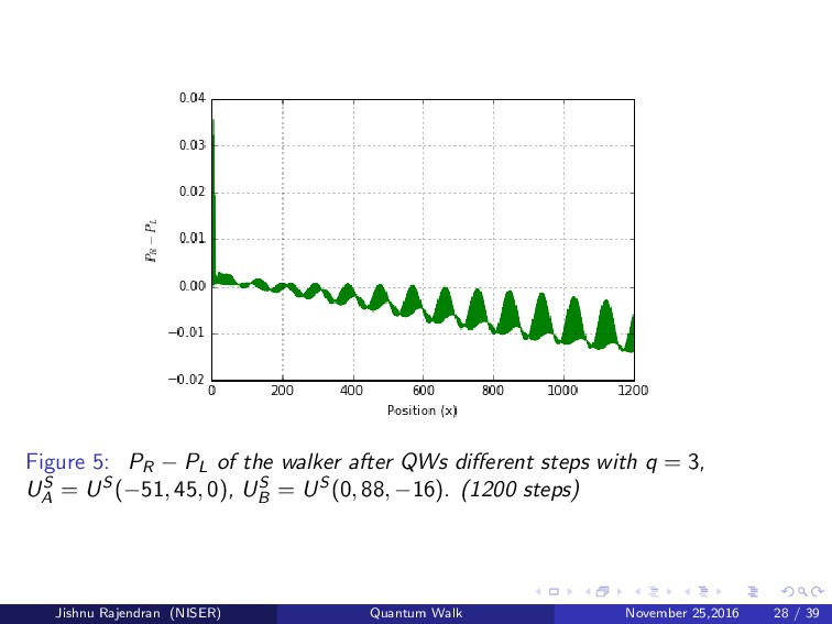
27. Figure 4: PR − PL of the walker after QWs different steps with q = 3, US A = US (−51, 45, 0), US B = US (0, 88, −16). (first 250 steps) Jishnu Rajendran (NISER) Quantum Walk November 25,2016 27 / 39
28. Figure 5: PR − PL of the walker after QWs different steps with q = 3, US A = US (−51, 45, 0), US B = US (0, 88, −16). (1200 steps) Jishnu Rajendran (NISER) Quantum Walk November 25,2016 28 / 39
29. Outcome From the graphs we can see that the winning outcome is transient in nature,in asymptotic limits the game yields a losing strategy. So for large enough steps the game will loss. Jishnu Rajendran (NISER) Quantum Walk November 25,2016 29 / 39
30. Comparing Classical and quantum Parrondo’s games Jishnu Rajendran (NISER) Quantum Walk November 25,2016 30 / 39
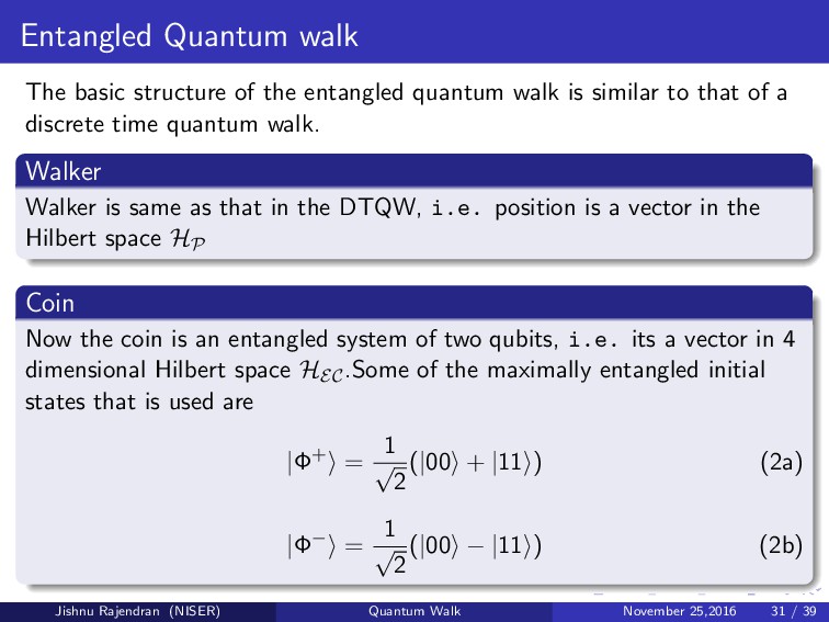
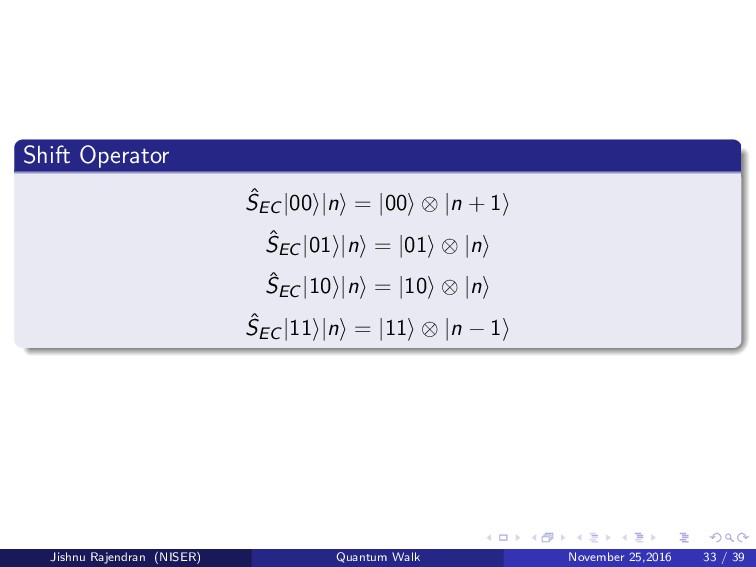
31. Entangled Quantum walk The basic structure of the entangled quantum walk is similar to that of a discrete time quantum walk. Walker Walker is same as that in the DTQW, i.e. position is a vector in the Hilbert space HP Coin Now the coin is an entangled system of two qubits, i.e. its a vector in 4 dimensional Hilbert space HEC.Some of the maximally entangled initial states that is used are |Φ+ = 1 √ 2 (|00 + |11 ) (2a) |Φ− = 1 √ 2 (|00 − |11 ) (2b) Jishnu Rajendran (NISER) Quantum Walk November 25,2016 31 / 39
32. Evolution Operator The evolution is defined as the tensor product of the two single-qubit coin operators We define the unbiased coin operator as the tensor product ˆ H⊗2 So ˆ CH EC in matrix form is ˆ CH EC = 1 2     1 1 1 1 1 −1 1 −1 1 1 −1 −1 1 −1 −1 1     Jishnu Rajendran (NISER) Quantum Walk November 25,2016 32 / 39
33. Shift Operator ˆ SEC |00 |n = |00 ⊗ |n + 1 ˆ SEC |01 |n = |01 ⊗ |n ˆ SEC |10 |n = |10 ⊗ |n ˆ SEC |11 |n = |11 ⊗ |n − 1 Jishnu Rajendran (NISER) Quantum Walk November 25,2016 33 / 39
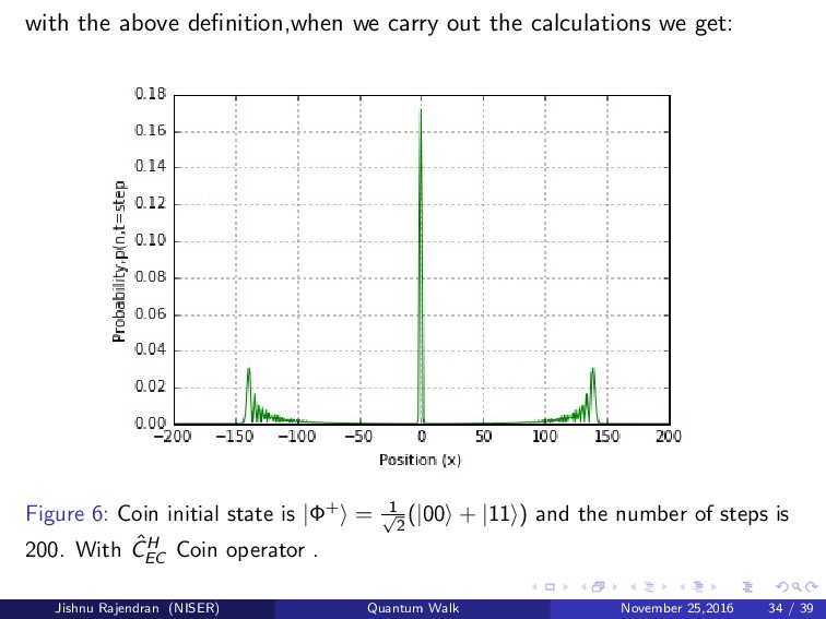
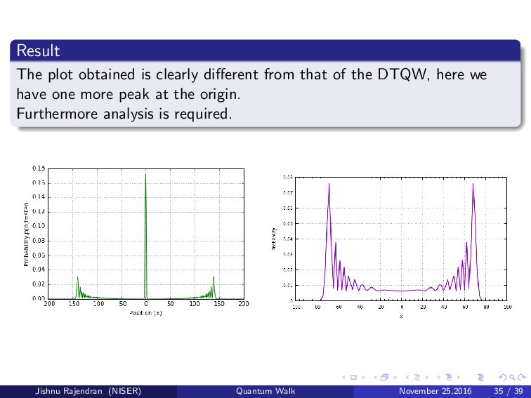
34. with the above definition,when we carry out the calculations we get: Figure 6: Coin initial state is |Φ+ = 1 √ 2 (|00 + |11 ) and the number of steps is 200. With ˆ CH EC Coin operator . Jishnu Rajendran (NISER) Quantum Walk November 25,2016 34 / 39
35. Result The plot obtained is clearly different from that of the DTQW, here we have one more peak at the origin. Furthermore analysis is required. Jishnu Rajendran (NISER) Quantum Walk November 25,2016 35 / 39
36. Entangled Parrondo’s quantum walk Entangled Parrondo’s quantum walk Now that the outcome of the entangled quantum walk is different from DTQW.We would investigate how it can affect the Parronodo’s games. How does it affect the paradox ?. Here we will consider a pair of entangled coins. They will acting upon the state in an alternating fashion. This is yet to be done and the result will be reported in the manuscript: Playing Parrondo’s game in an Entangled quantum walk, Jishnu Rajendran,Colin Benjamin Jishnu Rajendran (NISER) Quantum Walk November 25,2016 36 / 39
37. Conclusion From the motivation of classical random walk we studied quantum walk. The non-intuitive nature of parrondo’s games classically. Nature of parrondo’s games in a quantum scenario. Introducing entanglement in quantum walk and its behavior. Outlook Introducing entanglement to the quantum version of parrondo’s games. Jishnu Rajendran (NISER) Quantum Walk November 25,2016 37 / 39
38. Reference (1) Quantum Walks and Search Algorithms ,Renato Portugal (2) J. Kempe,Quantum random walks - an introductory overview, Contemporary Physics, 44(4), 307 (2003). (3) S. E. Venegas-Andraca, Quantum walks: a comprehensive review (2012) 11:1015-1106. (4) M. Li, Y. S. Zhang and G. C. Guo, Qunatum Parrondo’s games constructed by quantum random walk, 30, 020304 (2013). (5)A. P. Flitney,Quantum Parrondo’s games using quantum walks, arXiv:quant-ph/1209.2252 (2012). Jishnu Rajendran (NISER) Quantum Walk November 25,2016 38 / 39
39. The end of this presentation Thank You All Jishnu Rajendran (NISER) Quantum Walk November 25,2016 39 / 39