STOCHASTIC METHODS FOR INFLATION MODEL BUILDING

Talk given at the University of Amsterdam

Transcript

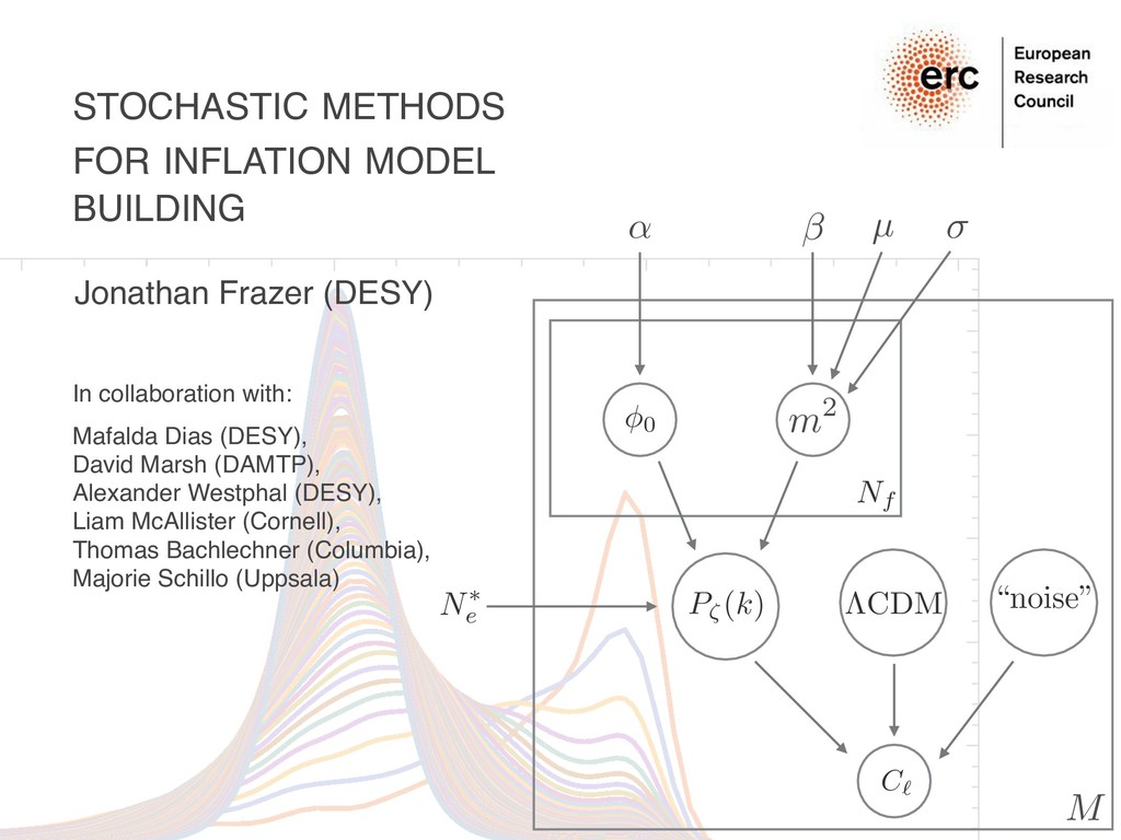
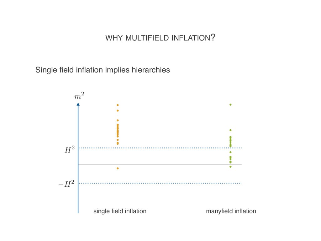
1. In collaboration with: Mafalda Dias (DESY), David Marsh (DAMTP), Alexander Westphal (DESY), Liam McAllister (Cornell), Thomas Bachlechner (Columbia), Majorie Schillo (Uppsala) Jonathan Frazer (DESY) STOCHASTIC METHODS FOR INFLATION MODEL BUILDING M C` Nf 0 m2 ↵ P⇣(k) N⇤ e “noise” ⇤CDM µ
2. OVERVIEW 1. Introduction to multifield inflation 2. Viewing complexity as an opportunity rather than a problem 3. Example 1: N-flation 4. Example 2: DBM inflation 5. Can we improve predictions with a stochastic approach? 6. A (Bayesian) network perspective on inflation 7. Outlook
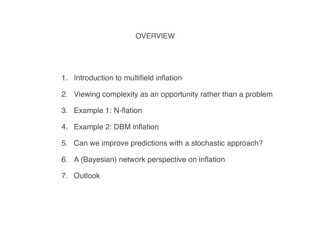
3. INFLATION SEEDS STRUCTURE FORMATION C` = Z d ln k P⇣(k)T2 ` (k) Angular power spectrum of CMB temperature fluctuations Transfer function — depends only on known physics Power spectrum of density fluctuations at the moment of horizon reentry
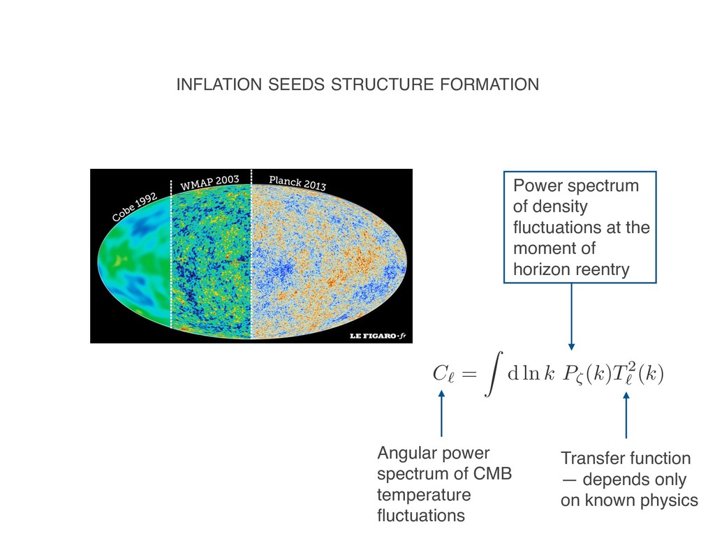
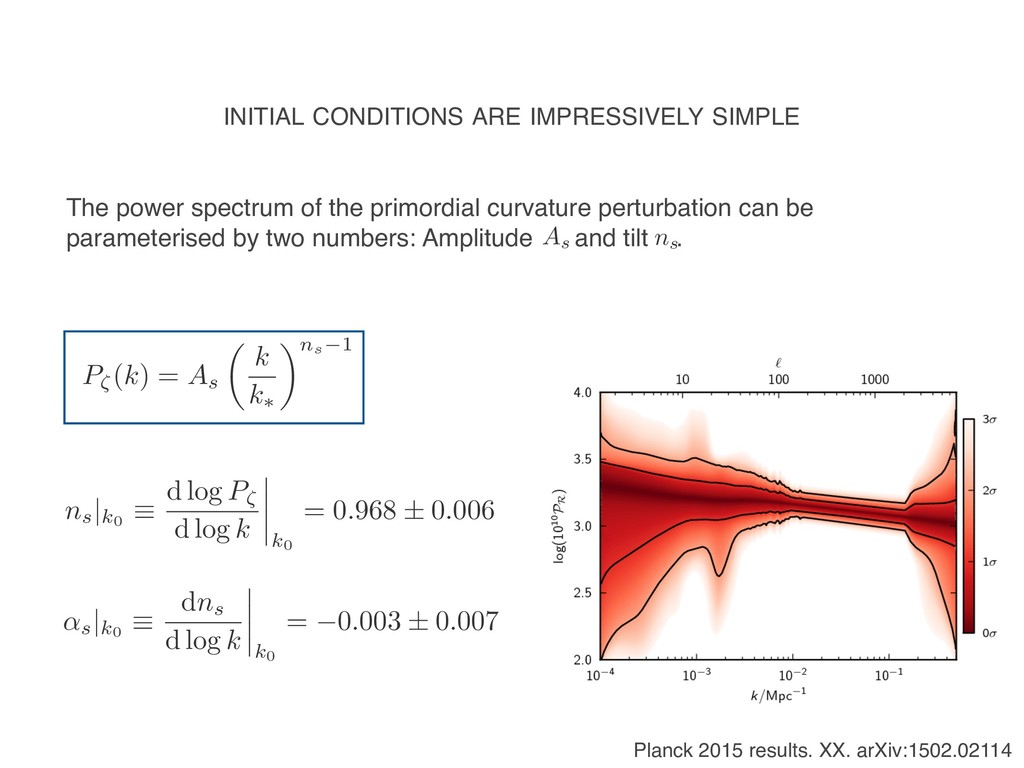
4. t reconstructions of the primordial power spectrum PR (k) using Planck TT data. The plot R (k)|k, N) for a given number of knots. The number of internal knots Nint increases (left to each k-slice, equal colours have equal probabilities. The colour scale is chosen so that dark nce intervals. 1 and 2 confidence intervals are also sketched (black curves). The upper h esponding multipoles via ` ⇡ k/Drec , where Drec is the comoving distance to recombination TT TTTEEE TT, reduced priors ns |k0 ⌘ d log P⇣ d log k k0 = 0.968 ± 0.006 ↵s |k0 ⌘ dns d log k k0 = 0.003 ± 0.007 Planck 2015 results. XX. arXiv:1502.02114 INITIAL CONDITIONS ARE IMPRESSIVELY SIMPLE P⇣(k) = As ✓ k k⇤ ◆ns 1 The power spectrum of the primordial curvature perturbation can be parameterised by two numbers: Amplitude and tilt . As ns
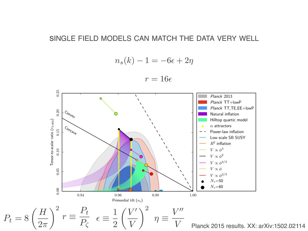
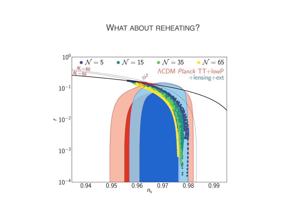
5. Fig. 11. Marginalized joint 68 % and 95 % CL regions for (✏1 , ✏2 , ✏3 ) (top panels) and (✏V , ⌘V , ⇠2 V ) (bottom panels) for Planck TT+lowP (red contours), Planck TT,TE,EE+lowP (blue contours), and compared with the Planck 2013 results (grey contours). Fig. 12. Marginalized joint 68 % and 95 % CL regions for ns and r0.002 from Planck in combination with other data sets, compared to the theoretical predictions of selected inflationary models. Planck 2015 results. XX: arXiv:1502.02114 ns(k) 1 = 6✏ + 2⌘ r = 16✏ sINGLE FIELD MODELS CAN MATCH THE DATA VERY WELL r ⌘ Pt P⇣ Pt = 8 ✓ H 2⇡ ◆2 ⌘ ⌘ V 00 V ✏ ⌘ 1 2 ✓ V 0 V ◆2
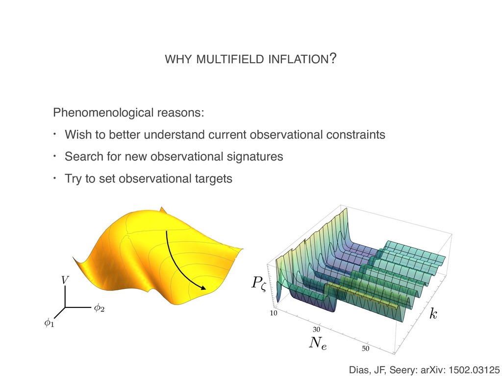
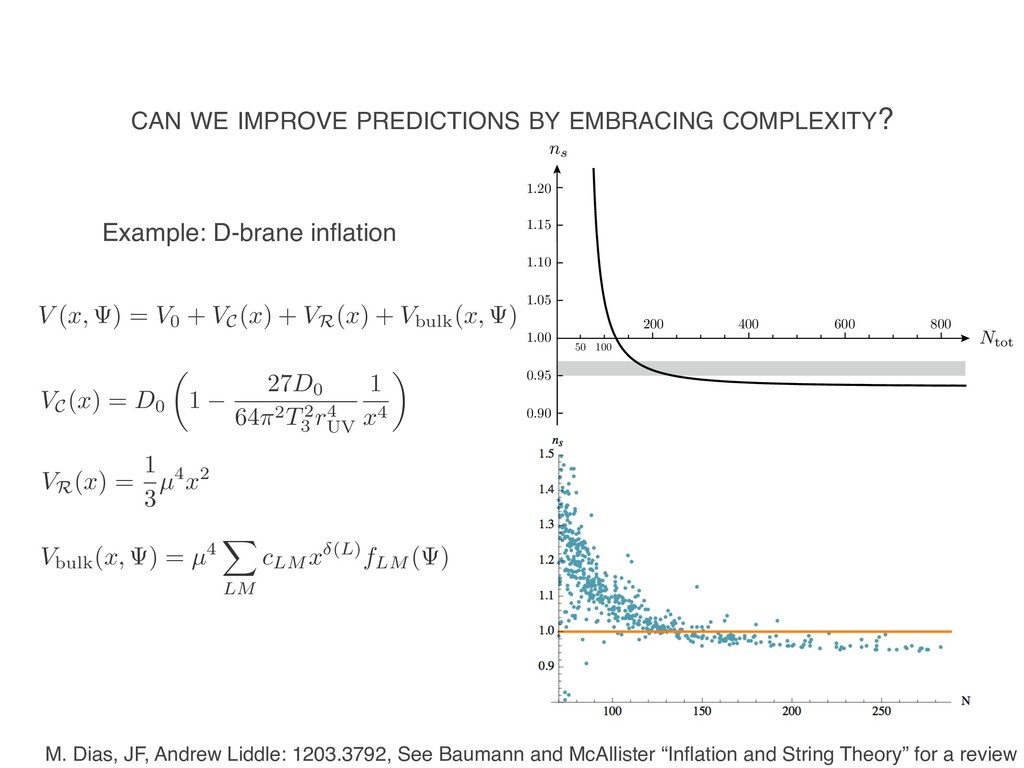
6. WHY MULTIFIELD INFLATION? Phenomenological reasons: • Wish to better understand current observational constraints • Search for new observational signatures • Try to set observational targets Dias, JF, Seery: arXiv: 1502.03125 1 2 V 30 50 10 P⇣ Ne k
7. WHY MULTIFIELD INFLATION? Phenomenological reasons: • Wish to better understand current observational constraints • Search for new observational signatures • Try to set observational targets Examples: The Lyth bound Maldacena’s consistency relation MPl & ⇣ r 0.01 ⌘1 2 flocal NL ⇡ 5 12 (ns 1) Surveys: AdvACT, CLASS, Keck/BICEP3 SPT-S3, CMBpol Euclid, LSST
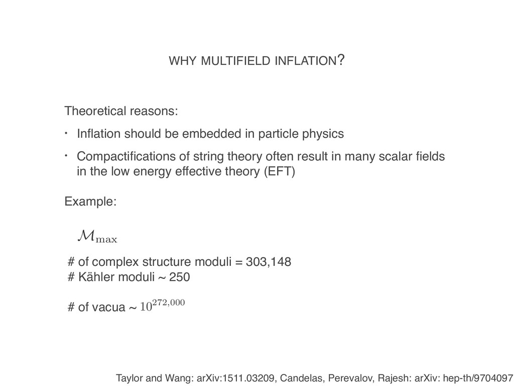
8. WHY MULTIFIELD INFLATION? Theoretical reasons: • Inflation should be embedded in particle physics • Compactifications of string theory often result in many scalar fields in the low energy effective theory (EFT) Example: # of complex structure moduli = 303,148 # Kähler moduli ~ 250 # of vacua ~ Mmax 10272,000 Taylor and Wang: arXiv:1511.03209, Candelas, Perevalov, Rajesh: arXiv: hep-th/9704097
9. WHY MULTIFIELD INFLATION? Single field inflation implies hierarchies single field inflation manyfield inflation m2 H 2 H 2
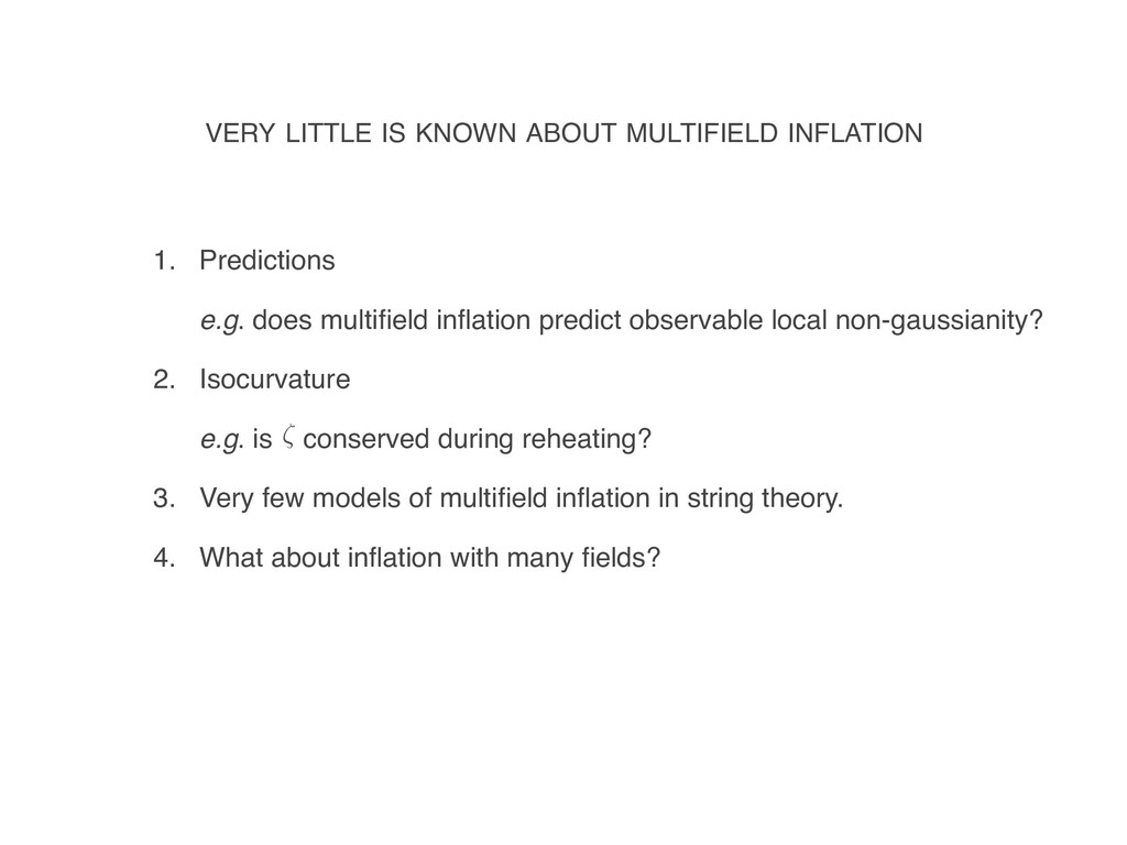
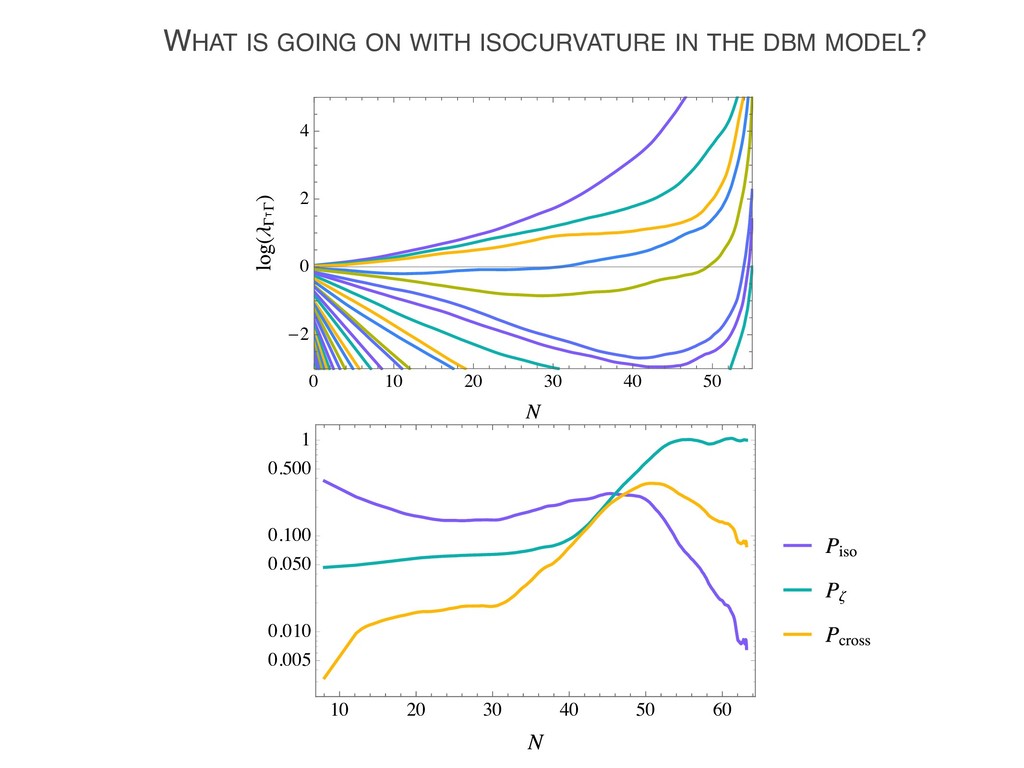
10. VERY LITTLE IS KNOWN ABOUT MULTIFIELD INFLATION 1. Predictions e.g. does multifield inflation predict observable local non-gaussianity? 2. Isocurvature e.g. is conserved during reheating? 3. Very few models of multifield inflation in string theory. 4. What about inflation with many fields? ⇣
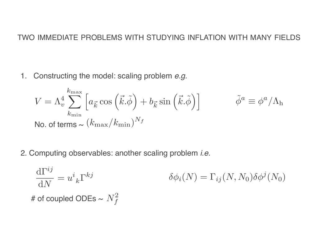
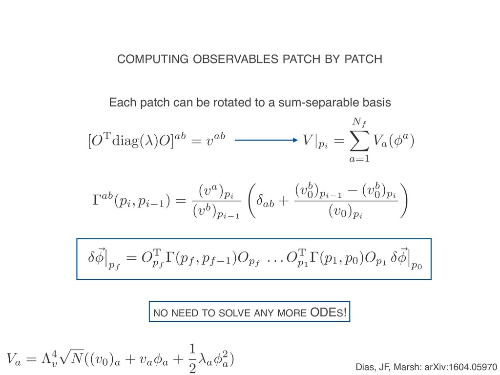
11. TWO IMMEDIATE PROBLEMS WITH STUDYING INFLATION WITH MANY FIELDS 1. Constructing the model: scaling problem e.g. 2. Computing observables: another scaling problem i.e. V = ⇤4 v kmax X kmin h a~ k cos ⇣ ~ k.˜ ⌘ + b~ k sin ⇣ ~ k.˜ ⌘i (kmax/kmin)Nf No. of terms ~ # of coupled ODEs ~ N2 f ˜a ⌘ a/⇤h d ij dN = ui k kj i(N) = ij(N, N0) j(N0)
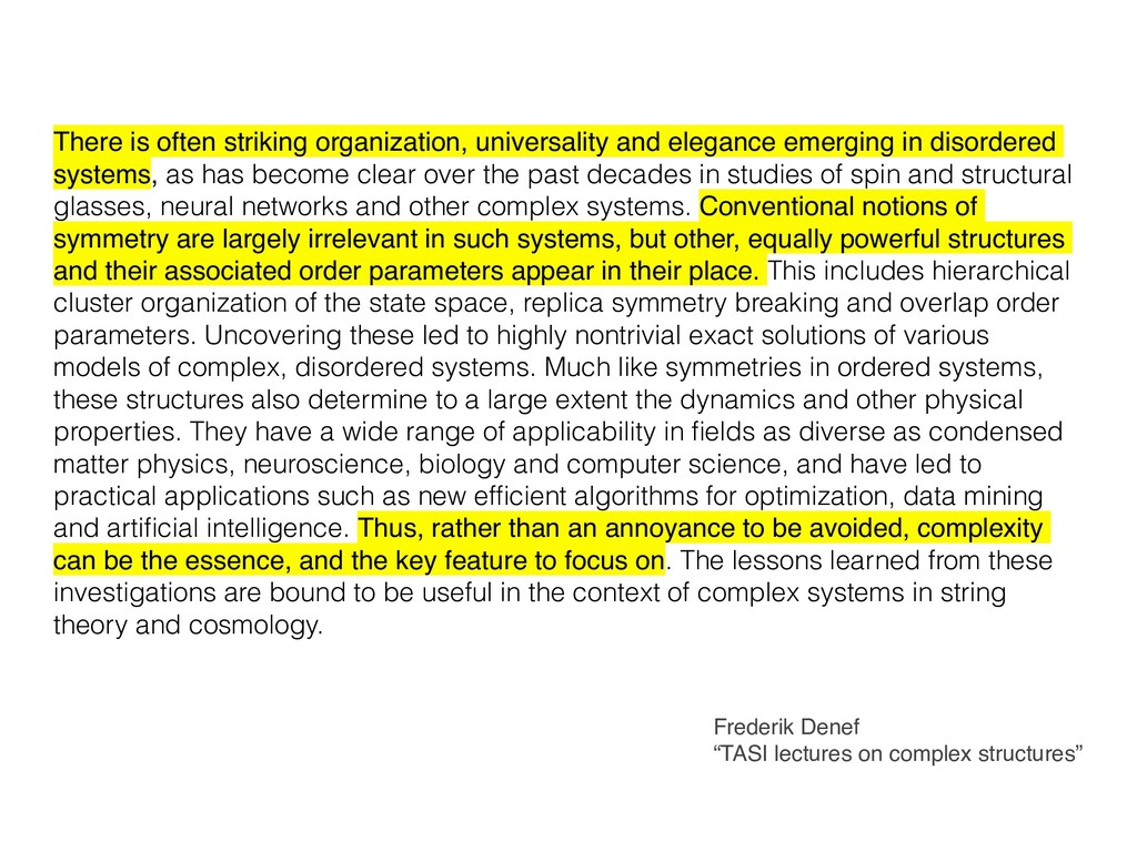
12. There is often striking organization, universality and elegance emerging in disordered systems, as has become clear over the past decades in studies of spin and structural glasses, neural networks and other complex systems. Conventional notions of symmetry are largely irrelevant in such systems, but other, equally powerful structures and their associated order parameters appear in their place. This includes hierarchical cluster organization of the state space, replica symmetry breaking and overlap order parameters. Uncovering these led to highly nontrivial exact solutions of various models of complex, disordered systems. Much like symmetries in ordered systems, these structures also determine to a large extent the dynamics and other physical properties. They have a wide range of applicability in fields as diverse as condensed matter physics, neuroscience, biology and computer science, and have led to practical applications such as new efficient algorithms for optimization, data mining and artificial intelligence. Thus, rather than an annoyance to be avoided, complexity can be the essence, and the key feature to focus on. The lessons learned from these investigations are bound to be useful in the context of complex systems in string theory and cosmology. Frederik Denef “TASI lectures on complex structures”
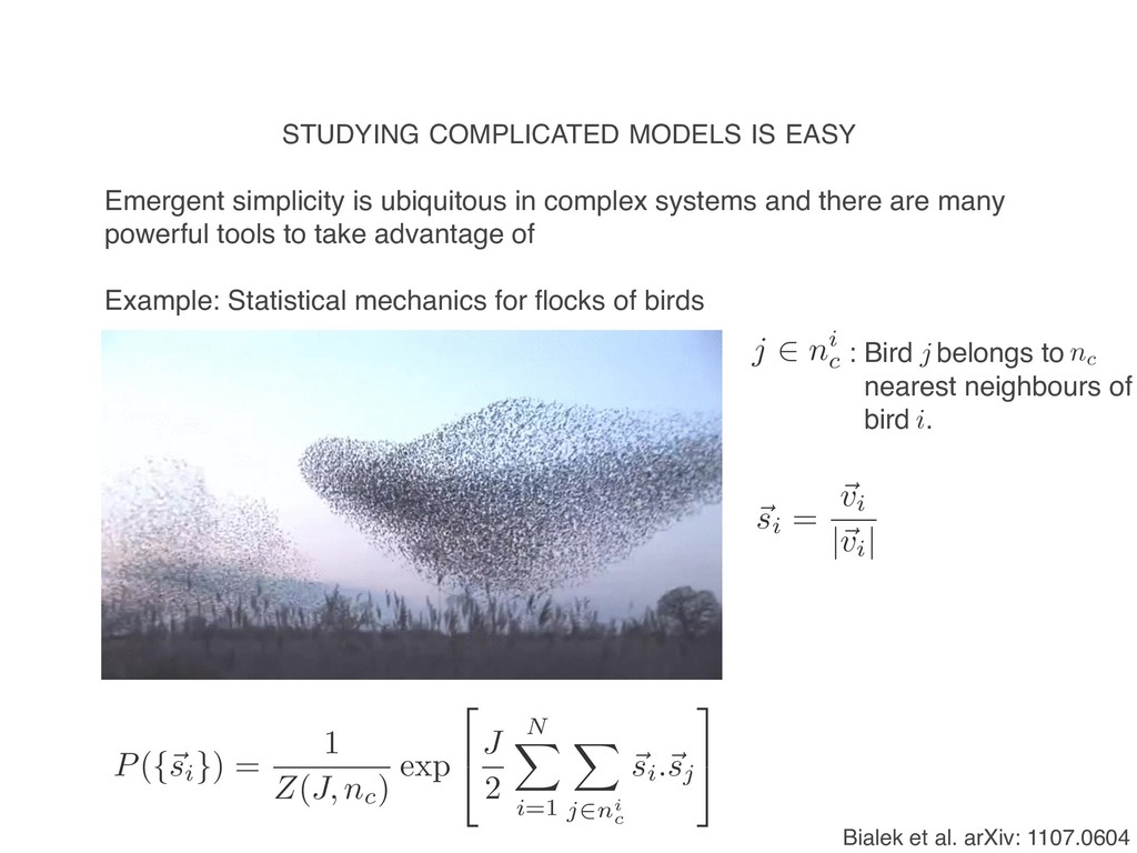
13. STUDYING COMPLICATED MODELS IS EASY Emergent simplicity is ubiquitous in complex systems and there are many powerful tools to take advantage of Example: Statistical mechanics for flocks of birds P({~ si }) = 1 Z(J, nc) exp 2 4J 2 N X i=1 X j2ni c ~ si.~ sj 3 5 j 2 ni c : Bird belongs to nearest neighbours of bird . i j nc ~ si = ~ vi |~ vi | Bialek et al. arXiv: 1107.0604
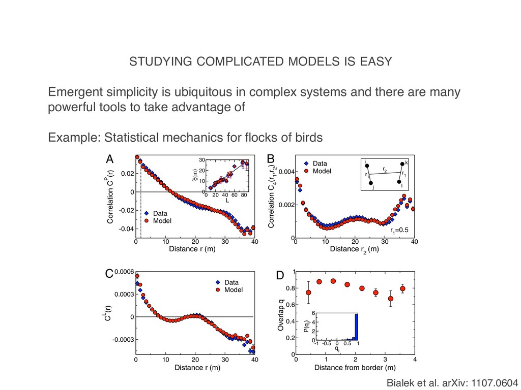
14. STUDYING COMPLICATED MODELS IS EASY 0 10 20 30 40 Distance r (m) -0.04 -0.02 0 0.02 Correlation CP (r) Data Model 0 20 40 60 80 L 0 10 20 30 (m) A 0 10 20 30 40 Distance r 2 (m) 0 0.002 0.004 Correlation C 4 (r 1 ,r 2 ) r 1 =0.5 Data Model i j l k r 1 r 2 r 1 B 0 10 20 30 40 Distance r (m) -0.0003 0 0.0003 0.0006 CL (r) C Data Model -1 -0.5 0 0.5 1 q i 0 2 4 6 P(q i ) D 0 1 2 3 4 Distance from border (m) 0 0.2 0.4 0.6 0.8 1 Overlap q Fig. 3. Correlation functions predicted by the maximum entropy model vs. experiment. The full pair correlation function can be written in terms of a long- Bialek et al. arXiv: 1107.0604 Emergent simplicity is ubiquitous in complex systems and there are many powerful tools to take advantage of Example: Statistical mechanics for flocks of birds
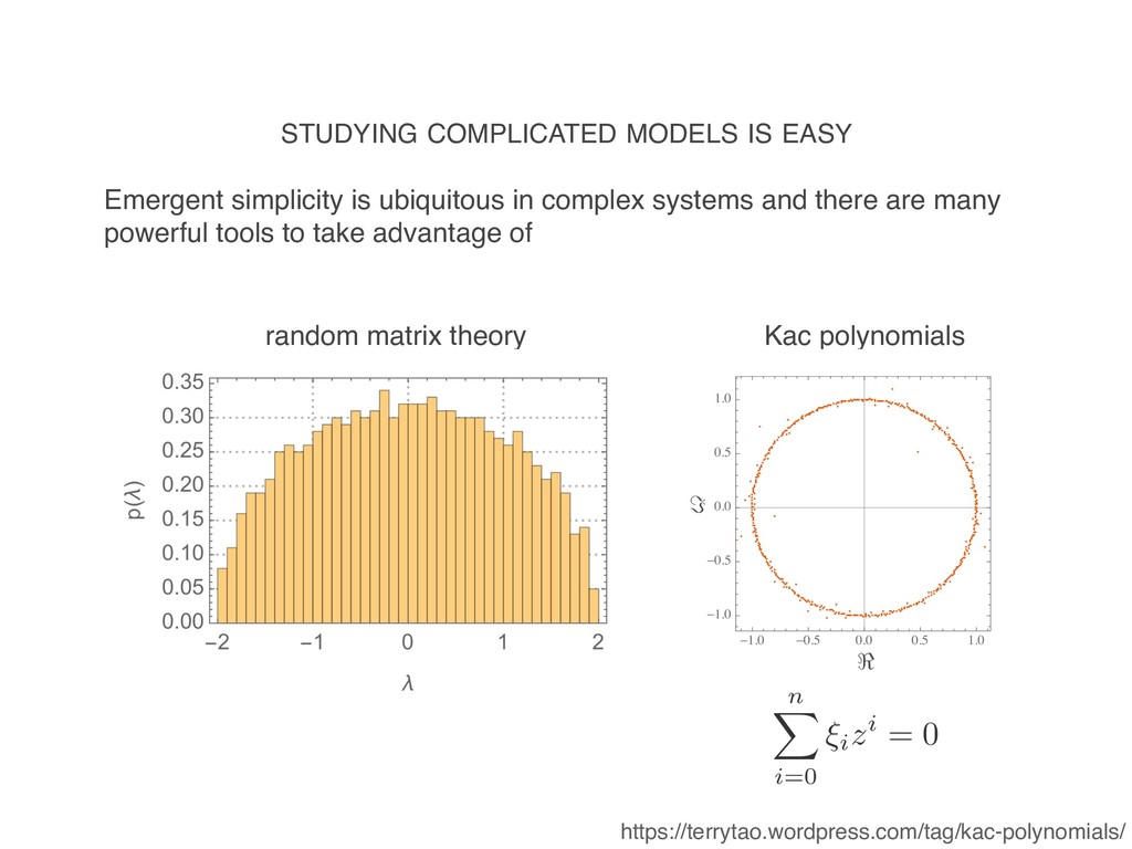
15. STUDYING COMPLICATED MODELS IS EASY Emergent simplicity is ubiquitous in complex systems and there are many powerful tools to take advantage of < = n X i=0 ⇠izi = 0 random matrix theory Kac polynomials https://terrytao.wordpress.com/tag/kac-polynomials/
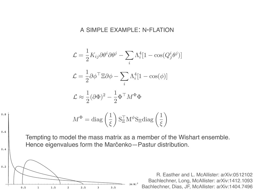
16. A SIMPLE EXAMPLE: N-FLATION L = 1 2 Kij@✓i@✓j X i ⇤4 i [1 cos(Qi j ✓j)] L = 1 2 @ >⌅@ X i ⇤4 i [1 cos( )] M = diag ✓ 1 ⇠ ◆ S> ⌅ M S⌅diag ✓ 1 ⇠ ◆ L ⇡ 1 2 (@ )2 1 2 >M Tempting to model the mass matrix as a member of the Wishart ensemble. Hence eigenvalues form the Marčenko—Pastur distribution. R. Easther and L. McAllister: arXiv:0512102 Bachlechner, Long, McAllister: arXiv:1412.1093 Bachlechner, Dias, JF, McAllister: arXiv:1404.7496 0.5 1 1.5 2 2.5 3 3.5 m m 2 0.2 0.4 0.6 0.8 ive probability