Upgrade to Pro — share decks privately, control downloads, hide ads and more …

Manyfield Inflation

Manyfield Inflation

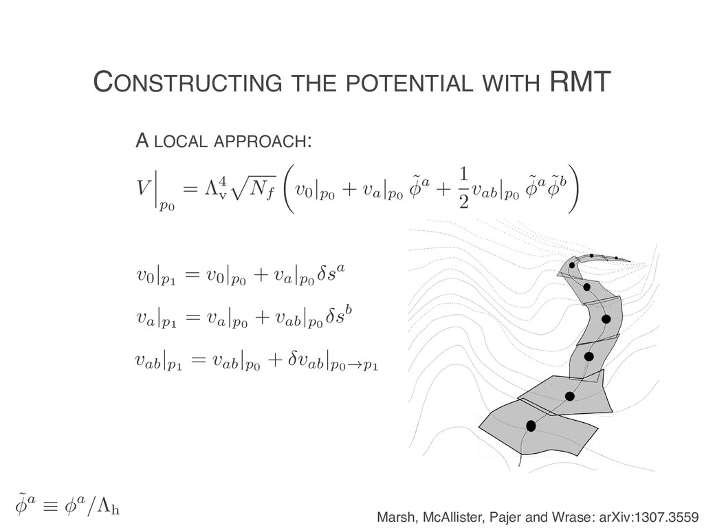
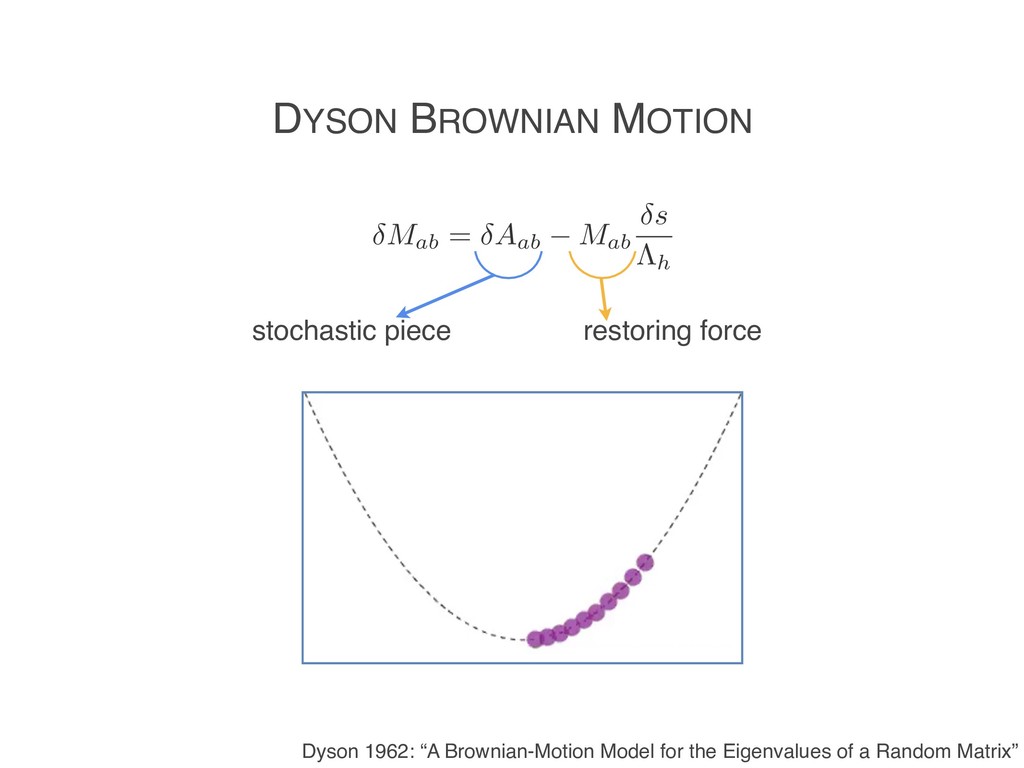
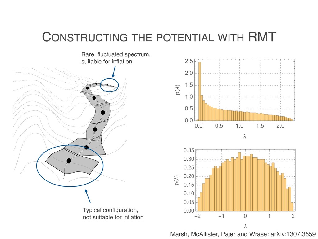
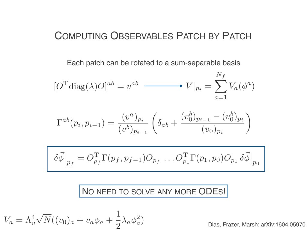
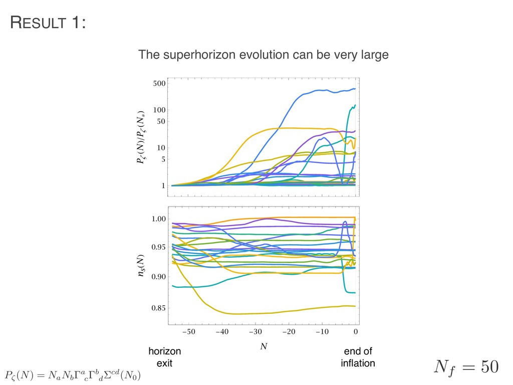
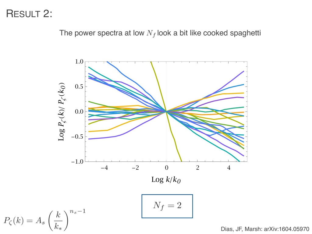
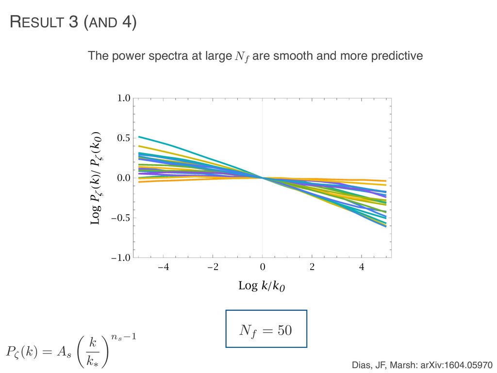
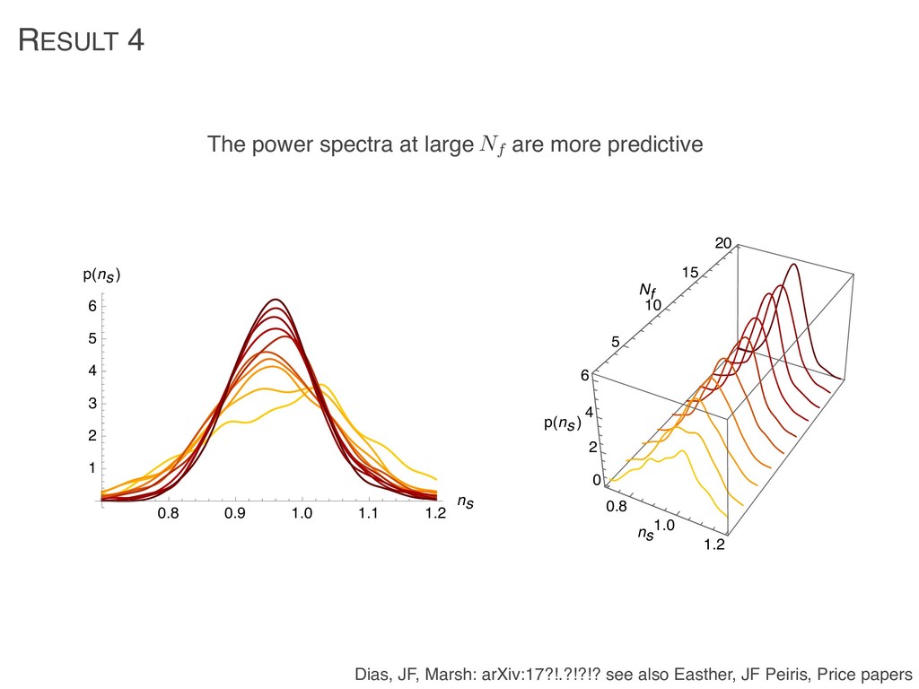
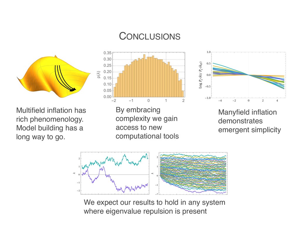
Work presented at the 3-PAC seminar series in Imperial College London in 2017. I don't remember what the abstract was but it would have been something about our work using Dyson Brownian Motion to study inflation with a very large number of scalar degrees of freedom. Our main result was that we found emergent simplicity at the level of cosmological predictions.

Jonathan Frazer

March 13, 2017
Tweet

More Decks by Jonathan Frazer

Other Decks in Research

Transcript

  1. 0.5 1.0 1.5 DfêLh Jonathan Frazer (DESY) In collaboration with

    Mafalda Dias (DESY), David Marsh (DAMTP), Alexander Westphal (DESY), David Seery (Sussex), David Mulryne (QMUL), Liam McAllister (Cornell), Thomas Bachlechner (Columbia), Layne Price (Amazon), Hiranya Peiris (UCL), Richard Easther (Auckland) MANYFIELD INFLATION
  2. OVERVIEW 1. Inflation - from (very) high energy physics to

    cosmology 2. What did we learn from the Planck satellite? 3. Multifield Inflation - why care? 4. Why complex models are complex 5. Why complex models are simple 6. Random Matrix Theory (RMT) 7. Inflation with Dyson Brownian Motion (DBM) 8. Some results
  3. INFLATION d dt (aH) 1 < 0 ) ✏ ⌘

    ˙ H H2 < 1 , d2 a dt2 > 0 Shrinking Hubble radius Slowly varying Hubble parameter Accelerated expansion H ⌘ ˙ a a ds2 = dt2 + a(t)2dx2 scale factor
  4. INFLATION d dt (aH) 1 < 0 ) ✏ ⌘

    ˙ H H2 < 1 , d2 a dt2 > 0 Quantum mechanical processes during inflation seed a distribution of gravitational potential wells As matter sank into these wells it formed the largest structures we see today The consequence is that any observable tracing this structure can be used to infer details of the seeding process
  5. INFLATION 1.3 The Shrinking Hubble Sphere 1 super-horizon sub-horizon CMB

    recombination today time comoving scales horizon re-entry sub-horizon horizon exit (aH) 1 k 1 reheating INFLATION [ln a] ure 1.3: Solution of the horizon problem. Scales of cosmological interest were larger than t 5 d dt (aH) 1 < 0 ) ✏ ⌘ ˙ H H2 < 1 , d2 a dt2 > 0
  6. INFLATION Example: The Cosmic Microwave Background (CMB) C` = Z

    d ln k P⇣(k)T2 ` (k) Angular power spectrum of CMB temperature fluctuations Transfer function — depends only on known physics Power spectrum of density fluctuations at the moment of horizon reentry
  7. t reconstructions of the primordial power spectrum PR (k) using

    Planck TT data. The plot R (k)|k, N) for a given number of knots. The number of internal knots Nint increases (left to each k-slice, equal colours have equal probabilities. The colour scale is chosen so that dark nce intervals. 1 and 2 confidence intervals are also sketched (black curves). The upper h esponding multipoles via ` ⇡ k/Drec , where Drec is the comoving distance to recombination TT TTTEEE TT, reduced priors ns |k0 ⌘ d log P⇣ d log k k0 = 0.968 ± 0.006 ↵s |k0 ⌘ dns d log k k0 = 0.003 ± 0.007 Planck 2015 results. XX. arXiv:1502.02114 CURRENT CONSTRAINTS P⇣(k) = As ✓ k k⇤ ◆ns 1 The power spectrum of the primordial curvature perturbation can be parameterised by two numbers: Amplitude and tilt . As ns
  8. INFLATION Inflation is usually modelled as being driven by one

    or more scalar fields ¨ i + 3H ˙ i + @iV = 0 ✏ < 1 ) 1 2 ViV i V 2 < 1 S = Z d4x p g " M2 pl 2 R 1 2 @µ i@µ i V ( 1, . . . , Nf ) # 1 2 V V ( )
  9. INFLATION On superhorizon scales field perturbations can be thought of

    as forming a bundle of non-interacting trajectories When the slow-roll assumption holds, inflationary perturbation theory on superhorizon scales, is precisely analogous to geometrical optics 00 i + (3 ✏) 0 i + V,i H2 = 0 H 2 = V 3 ✏ 0 ⌘ d dN = 1 H d dt 0 i = ui ui ⌘ @i ln V ⌫ d i ds = @iS ⌫ ⌘ p 2✏ Huygen’s equation! Describes the propagation of a light ray in a medium with spatially varying refractive index refractive index D. Seery, D. Mulryne, JF, R. Ribiero 1203.2635
  10. INFLATION On superhorizon scales field perturbations can be thought of

    as forming a bundle of non-interacting trajectories When the slow-roll assumption holds, inflationary perturbation theory on superhorizon scales is precisely analogous to geometrical optics d i dN = uij j i(N) = ij(N, N0) j(N0) ij(N, N0) ⌘ P exp Z N N0 uij(N0)dN0 uij ⌘ @i@j ln V Gauge transformation D. Seery, D. Mulryne, JF, R. Ribiero 1203.2635 P⇣(N) = NiNj i k j l h k liN0 Ni ⌘ 1 2✏ Vi V
  11. INFLATION Example: Single field inflation ij(N, N0) ⌘ P exp

    Z N N0 uij(N0)dN0 P⇣(N) = NiNj i k j l h k liN0 ( I, F ) = exp "Z F I d V V 0 ✓ V 00 V 0 V 0 V ◆# = V 0 F VF VI V 0 I N0 = 1 p 2✏I Ni ⌘ 1 2✏ Vi V Conserved on superhorizon scales! P⇣ = 1 2✏I ✓ H 2⇡ ◆2 I V ( )
  12. Fig. 11. Marginalized joint 68 % and 95 % CL

    regions for (✏1 , ✏2 , ✏3 ) (top panels) and (✏V , ⌘V , ⇠2 V ) (bottom panels) for Planck TT+lowP (red contours), Planck TT,TE,EE+lowP (blue contours), and compared with the Planck 2013 results (grey contours). Fig. 12. Marginalized joint 68 % and 95 % CL regions for ns and r0.002 from Planck in combination with other data sets, compared to the theoretical predictions of selected inflationary models. Planck 2015 results. XX: arXiv:1502.02114 ns(k) 1 = 6✏ + 2⌘ r = 16✏ SIMPLEST INFLATION MODELS FIT DATA r ⌘ Pt P⇣ Pt = 8 ✓ H 2⇡ ◆2 ⌘ ⌘ V 00 V
  13. BICEP2 : arXiv:1510.09217 ns(k) 1 = 6✏ + 2⌘ r

    = 16✏ SIMPLEST INFLATION MODELS FIT DATA 2 0.95 0.96 0.97 0.98 0.99 1.00 ns 0.00 0.05 0.10 0.15 0.20 0.25 r0.002 N=50 N=60 Convex Concave Planck TT+lowP+lensing+ext +BK14 Sync upper limit 95x95 95x150 150x150 Ext noise uncer. Nominal band cente BB in l∼80 bandpower l(l+1)C l /2π [µK2] 0 50 100 150 200 10−4 10−3 10−2 10−1 100 101 FIG. 8. Expectation values and n the ` ⇠ 80 BB bandpower in the BIC solid and dashed black lines show the e of lensed-⇤CDM and r0.05 = 0.05. S used, the levels corresponding to these a r ⌘ Pt P⇣ Pt = 8 ✓ H 2⇡ ◆2 ⌘ ⌘ V 00 V
  14. WHY MULTIFIELD INFLATION? Phenomenological reasons: • Wish to better understand

    current observational constraints • Search for new observational signatures • Try to set observational targets 30 50 10 P⇣ Ne k Dias, JF, Seery: arXiv: 1502.03125
  15. WHY MULTIFIELD INFLATION? Phenomenological reasons: • Wish to better understand

    current observational constraints • Search for new observational signatures • Try to set observational targets Examples: The Lyth bound Maldacena’s consistency relation MPl & ⇣ r 0.01 ⌘1 2 flocal NL ⇡ 5 12 (ns 1) Surveys: AdvACT, CLASS, Keck/BICEP3 SPT-S3, CMBpol Euclid, LSST
  16. WHY MULTIFIELD INFLATION? Theoretical reasons: • Inflation should be embedded

    in particle physics • Compactifications of string theory often result in many scalar fields in the low energy effective theory (EFT) Example: # of complex structure moduli = 303,148 # Kähler moduli ~ 250 # of vacua ~ Mmax 10272,000 Taylor and Wang: arXiv:1511.03209, Candelas, Perevalov, Rajesh: arXiv: hep-th/9704097
  17. WHY MULTIFIELD INFLATION? Single field inflation implies hierarchies Generic point

    Single field inflation Manyfield inflation m2 H 2 H 2
  18. STUDYING COMPLICATED MODELS IS COMPLICATED Very little is known about

    inflation with many fields. Two challenges: 1. Constructing the model: scaling problem e.g. 2. Computing observables: another scaling problem i.e. V = ⇤4 v kmax X kmin h a~ k cos ⇣ ~ k.˜ ⌘ + b~ k sin ⇣ ~ k.˜ ⌘i (kmax/kmin)Nf No. of terms ~ # of coupled ODEs ~ N2 f ˜a ⌘ a/⇤h d ij dN = ui k kj
  19. STUDYING VERY COMPLICATED MODELS MIGHT BE SIMPLE Emergent simplicity is

    ubiquitous in complex systems and there are many powerful tools to take advantage of Example: Statistical mechanics for flocks of birds P({~ si }) = 1 Z(J, nc) exp 2 4J 2 N X i=1 X j2ni c ~ si.~ sj 3 5 j 2 ni c : Bird belongs to nearest neighbours of bird . i j nc ~ si = ~ vi |~ vi | Bialek et al. arXiv: 1107.0604
  20. STUDYING VERY COMPLICATED MODELS MIGHT BE SIMPLE 0 10 20

    30 40 Distance r (m) -0.04 -0.02 0 0.02 Correlation CP (r) Data Model 0 20 40 60 80 L 0 10 20 30 (m) A 0 10 20 30 40 Distance r 2 (m) 0 0.002 0.004 Correlation C 4 (r 1 ,r 2 ) r 1 =0.5 Data Model i j l k r 1 r 2 r 1 B 0 10 20 30 40 Distance r (m) -0.0003 0 0.0003 0.0006 CL (r) C Data Model -1 -0.5 0 0.5 1 q i 0 2 4 6 P(q i ) D 0 1 2 3 4 Distance from border (m) 0 0.2 0.4 0.6 0.8 1 Overlap q Fig. 3. Correlation functions predicted by the maximum entropy model vs. experiment. The full pair correlation function can be written in terms of a long- Bialek et al. arXiv: 1107.0604 Emergent simplicity is ubiquitous in complex systems and there are many powerful tools to take advantage of Example: Statistical mechanics for flocks of birds
  21. STUDYING VERY COMPLICATED MODELS MIGHT BE SIMPLE Emergent simplicity is

    ubiquitous in complex systems and there are many powerful tools to take advantage of < = n X i=0 ⇠izi = 0 Random Matrices Theory Kac polynomials https://terrytao.wordpress.com/tag/kac-polynomials/
  22. Random Matrix Theory: Gaussian Orthogonal Ensemble p(M)dM = p(M0)dM0 M

    0 = O T MO d ⇥ d entries are independent and identically distributed (iid)
  23. eigenvalue repulsion Random Matrix Theory: Gaussian Orthogonal Ensemble p( 1,

    . . . , n) = Ce 1 2 W W = 1 2 n X i=1 2 i X i6=j ln | i j | Eigenvalues behave like a gas of electrons in , confined to a line and subject to a quadratic potential R2 P( min > 0) / e N2 f D. S. Dean and S. N. Majumdar; cond-mat/0609651
  24. CONSTRUCTING THE POTENTIAL WITH RMT ˜a ⌘ a/⇤h Figure 1.

    By gluing nearby coordinate charts together, a potential along Marsh, McAllister, Pajer and Wrase: arXiv:1307.3559 A LOCAL APPROACH: V p0 = ⇤4 v p Nf ✓ v0 |p0 + va |p0 ˜a + 1 2 vab |p0 ˜a ˜b ◆ v0 |p1 = v0 |p0 + va |p0 sa va |p1 = va |p0 + vab |p0 sb vab |p1 = vab |p0 + vab |p0 !p1
  25. DYSON BROWNIAN MOTION Mab = Aab Mab s ⇤h stochastic

    piece restoring force Dyson 1962: “A Brownian-Motion Model for the Eigenvalues of a Random Matrix”
  26. ng nearby coordinate charts together, a potential along a path

    can be explored regions, so statistical properties of inflation in an ensemble be deduced by characterizing the potential along trajectories. Rare, fluctuated spectrum, suitable for inflation Typical configuration, not suitable for inflation CONSTRUCTING THE POTENTIAL WITH RMT Marsh, McAllister, Pajer and Wrase: arXiv:1307.3559
  27. NO NEED TO SOLVE ANY MORE ODES! COMPUTING OBSERVABLES PATCH

    BY PATCH Each patch can be rotated to a sum-separable basis ~ pf = O T pf (pf , pf 1)Opf . . . O T p1 (p1, p0)Op1 ~ p0 [O Tdiag( )O]ab = v ab ab(pi, pi 1) = (va)pi (vb)pi 1 ✓ ab + (vb 0 )pi 1 (vb 0 )pi (v0)pi ◆ Va = ⇤4 v p N((v0)a + va a + 1 2 a 2 a ) Dias, Frazer, Marsh: arXiv:1604.05970 V |pi = Nf X a=1 Va( a)
  28. FIG. 2: Superhorizon evolution of P⇣ (top) and ns (bottom)

    for the k0 mode, which leaves the horizon 55 e-folds before the end simplifies considerabl ns 1 Here, the unit vec throughout inflation, negligible component smallest eigenvalues contributions to ns . eigenvalues of vab|⇤ , est eigenvalue 1 , are variance of the spect initial patch, we can 1 as follows: at the so that to second ord k 1 = where cb0 = | 0 1 0 b ments of k 1 and then 1, s fixed), we find RESULT 1: P⇣(N) = NaNb a c b d ⌃cd(N0) Nf = 50 The superhorizon evolution can be very large horizon exit end of inflation
  29. rated ucted ) has , the nitial . In large

    e full and ram- at of ately or of va|p0 . s the ading d an on of -field on superhorizon scales is, up to numerical accuracy, zero (hence no plots are shown). All inflationary realisations considered here are of Dias, JF, Marsh: arXiv:1604.05970 RESULT 2: The power spectra at low look a bit like cooked spaghetti Nf Nf = 2 P⇣(k) = As ✓ k k⇤ ◆ns 1
  30. and ram- at of ately or of a|p0 . the

    ding d an n of field least cales e the 10 e- the am- iting agree FIG. 1: Example power spectra for the scales leaving the horizon between 50 and 60 e-folds before the end of inflation for Nf = 2 (top) and Nf = 50 (bottom), with ⇤h = 0.4. Dias, JF, Marsh: arXiv:1604.05970 RESULT 3 (AND 4) The power spectra at large are smooth and more predictive Nf P⇣(k) = As ✓ k k⇤ ◆ns 1 Nf = 50
  31. ��� ��� ��� ��� ��� �� � � � �

    � � �(�� ) ��� ��� ��� �� � �� �� �� �� � � � � �(�� ) RESULT 4 The power spectra at large are more predictive Nf Dias, JF, Marsh: arXiv:17?!.?!?!? see also Easther, JF Peiris, Price papers
  32. MORE PREDICTIVE SPECTRA : ANALYSE THE VARIANCE OF THE TILT

    n ab ⇤ ⌘ d⌃ d ln k ⇤ = ( ✏ ab u ab)⇤H 2 ⇤ ns 1 ⇡ 2eaeb ✓ vab v0⇤2 h ◆ ⇤ RANDOM MATRIX THEORY INTERPRETATION ns 1 = d ln P⇣ d ln k = 1 P⇣ NaNb a c b d ncd ⇤ The “predictivity” of the model is largely determined by the variance the smallest eigenvalue of the Hessian of the potential at horizon crossing
  33. ↵s ⇡ 4eaeb va c vcb v2 0 ⇤4 h

    ⇤ 4 ✓ eaebvab ⇤ v0⇤⇤2 h ◆2 + 2eaeb vab0 v0⇤2 h ⇤ ↵s = dns d ln k = 1 P⇣ NaNb a c b d↵cd ⇤ (ns 1)2 SMOOTHER SPECTRA : STUDY THE BEHAVIOUR OF THE RUNNING RANDOM MATRIX THEORY INTERPRETATION ↵ ab ⇤ ⌘ dnab d ln k ⇤ = [(2✏ 2 ✏ 0) ab u 0ab + 2✏u ab]⇤H 2 ⇤ 2[u a cn cb]⇤ Smoothness of the power spectra is largely determined by the volatility of the smallest eigenvalue of the Hessian of the potential at horizon crossing
  34. RANDOM MATRIX THEORY INTERPRETATION 0.0 0.5 1.0 1.5 2.0 -2

    -1 0 1 2 DfêLh l 0.0 0.5 1.0 1.5 2.0 -2 -1 0 1 2 DfêLh l Hence: How predictive the model is, as well as how smooth the spectra are, is determined by eigenvalue repulsion Dias, JF, Marsh: arXiv:1604.05970 p( 1, . . . , n) = Ce 1 2 W W = 1 2 n X i=1 2 i X i6=j ln | i j |
  35. conditions for the potential v0|p0 , va|p0 and vab|p0 .

    In this work we focus solely on e↵ects emerging from large Nf behaviour, leaving a more exhaustive study of the full parameter space to future work [16]. For the remaining parameters we take v0|p0 = 1, and chose va|p0 to set the initial value of the ✏ slow-roll param- eter. The initial spectrum of vab|p0 is chosen to be that of a fluctuated Wigner spectrum [19] with an approximately vanishing smallest eigenvalue, taking the eigenvector of the smallest eigenvalue of vab|p0 to be aligned with va|p0 . We note that eigenvalue repulsion quickly modifies the initial spectrum during Dyson Brownian Motion, leading to mass spectra with features on scales ⌧ ⇤h , and an insensitivity to the details of the initial distribution of vab [7]. The models we consider are then of small-field ‘approximate saddle-point’-type with ⇤h < MPl . Finally, for random potentials that give rise to at least 60 e-folds of inflation, we compute P⇣ (k) for the scales leaving the horizon between 50 and 60 e-folds before the end of inflation; assuming it is approximately this 10 e- fold range which is constrained by observations of the CMB. The ‘vertical scale’, ⇤v , is chosen to set the am- plitude of the power spectrum of the mode k0 exiting the horizon 55 e-folds before the end of inflation to agree with the COBE normalisation [20]. FIG. 1: Example power spectra for the scales leaving the horizon between 50 and 60 e-folds before the end of inflation for Nf = 2 (top) and Nf = 50 (bottom), with ⇤h = 0.4. 0.0 0.5 1.0 1.5 2.0 -2 -1 0 1 2 DfêLh l 0.0 0.5 1.0 1.5 2.0 -2 -1 0 1 2 DfêLh l CONCLUSIONS Multifield inflation has rich phenomenology. Model building has a long way to go. By embracing complexity we gain access to new computational tools Manyfield inflation demonstrates emergent simplicity We expect our results to hold in any system where eigenvalue repulsion is present