Typical Sets: What They Are and How to (Hopefully) Find Them

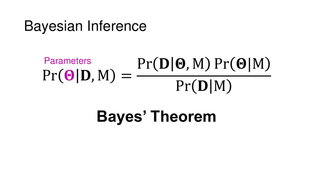
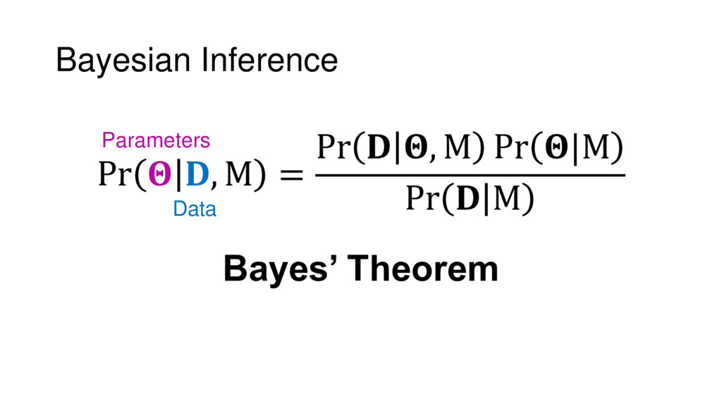
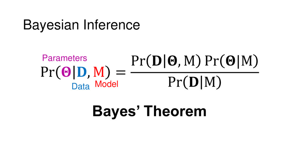
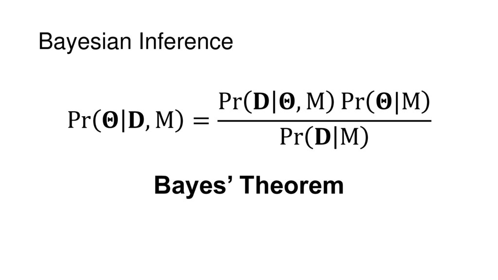
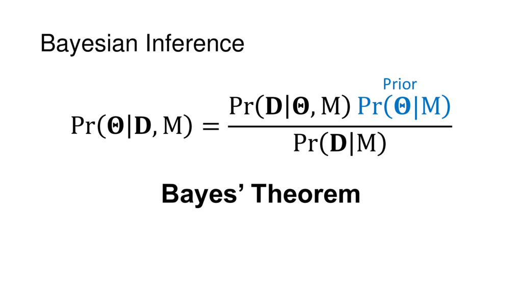
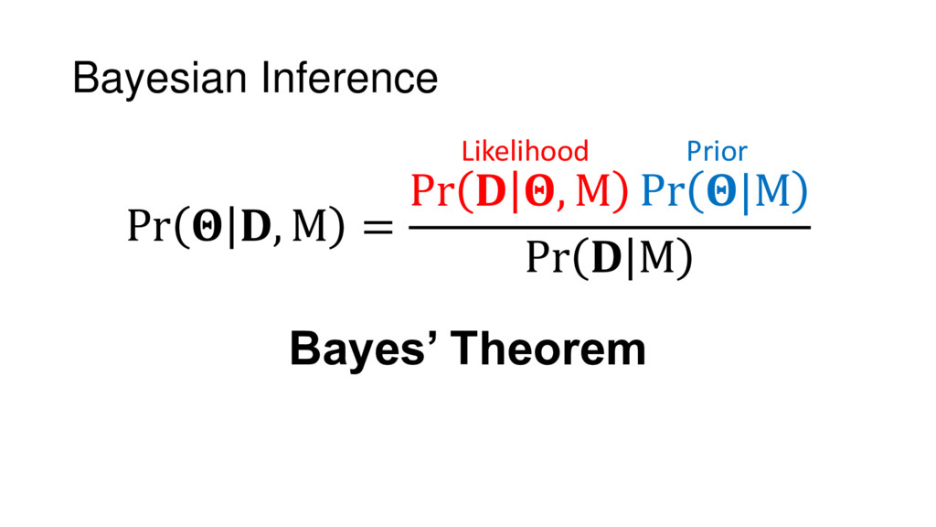
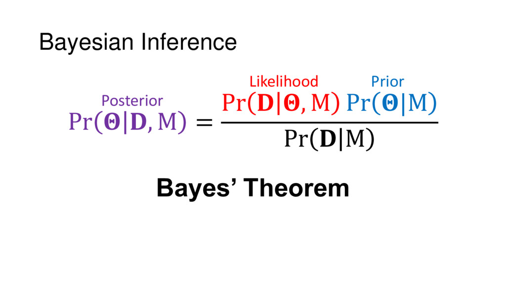
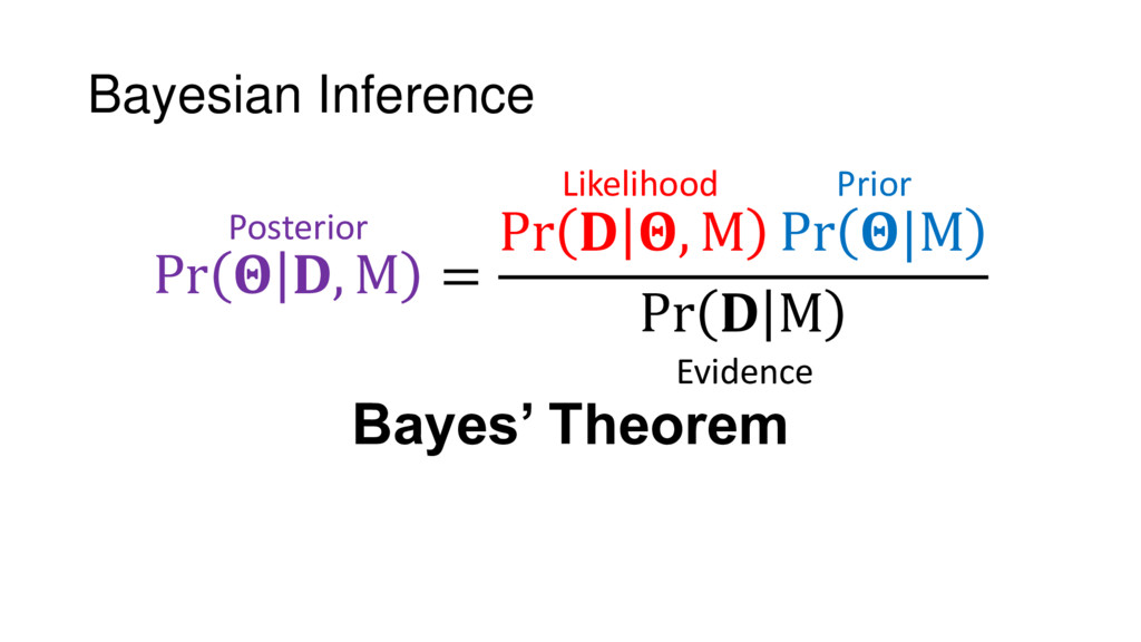
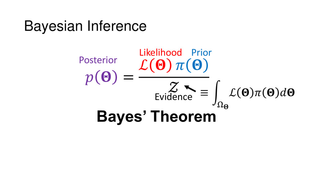
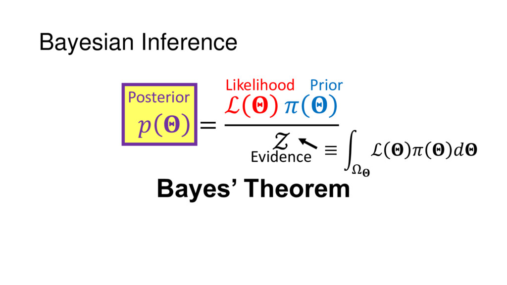
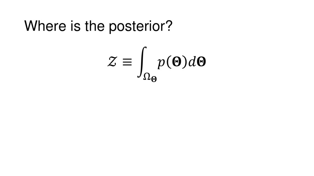
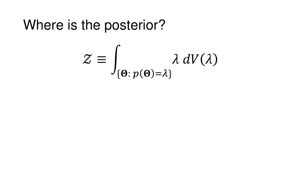
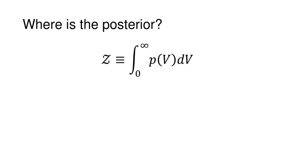
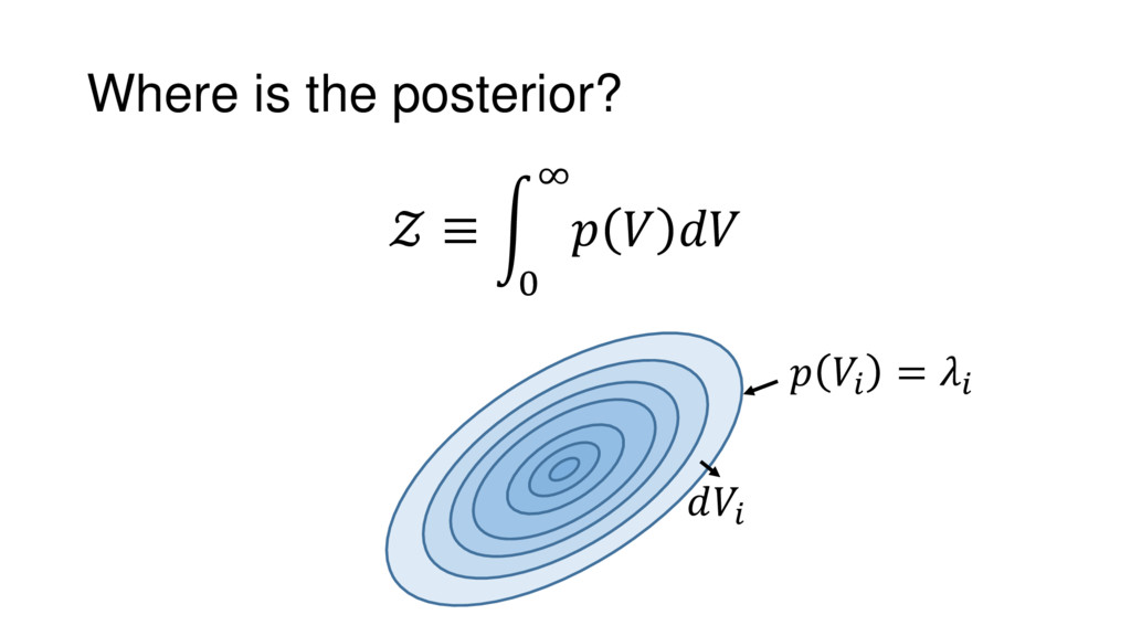
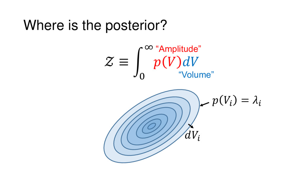
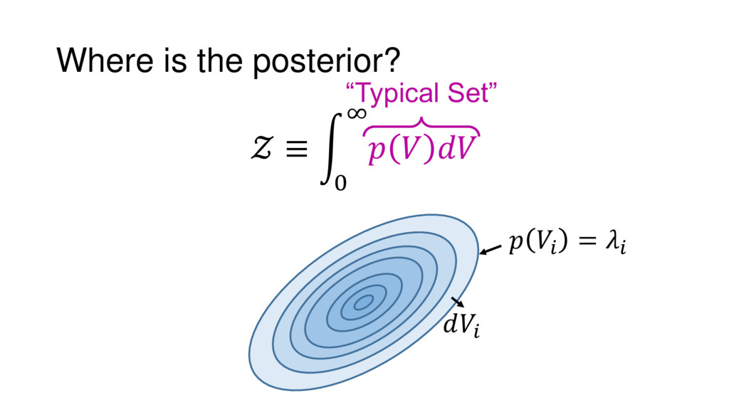
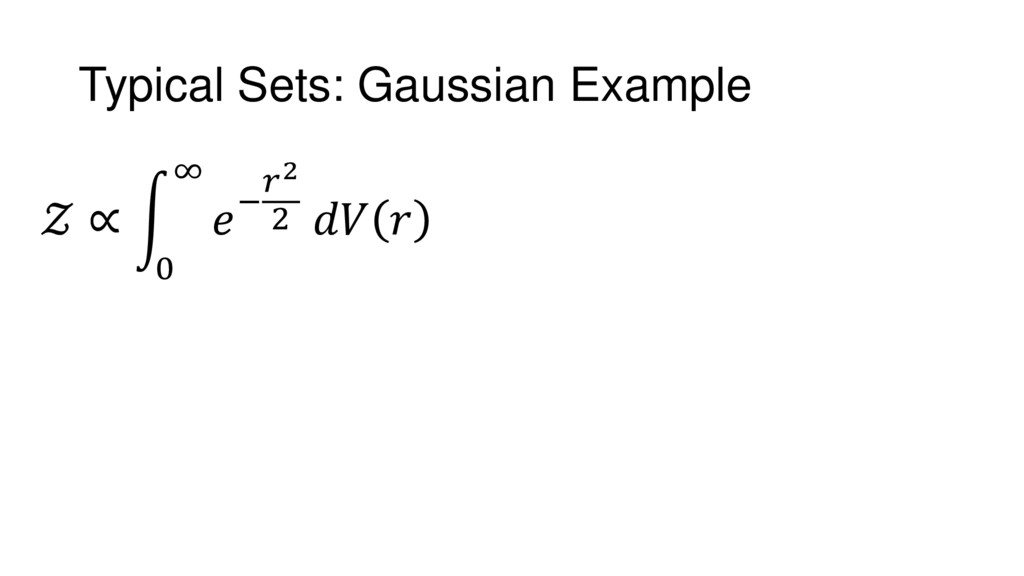
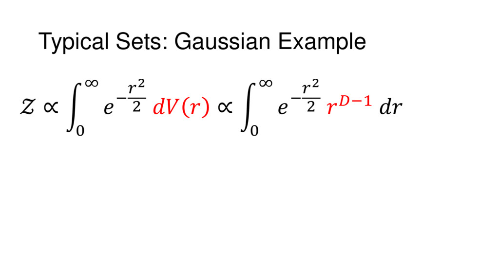
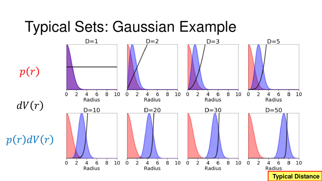
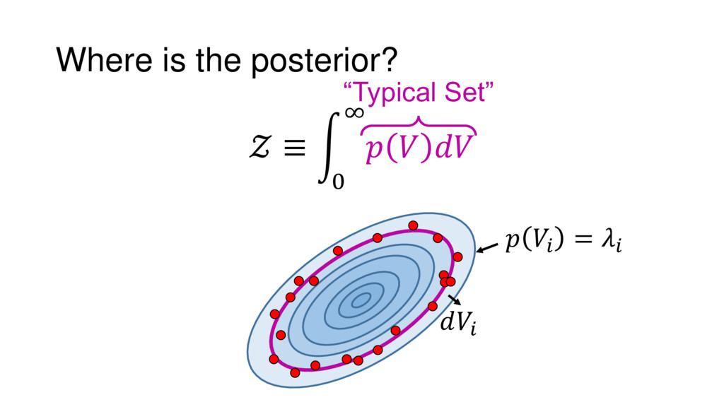
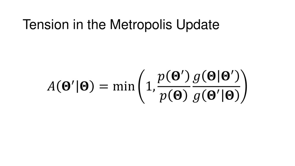
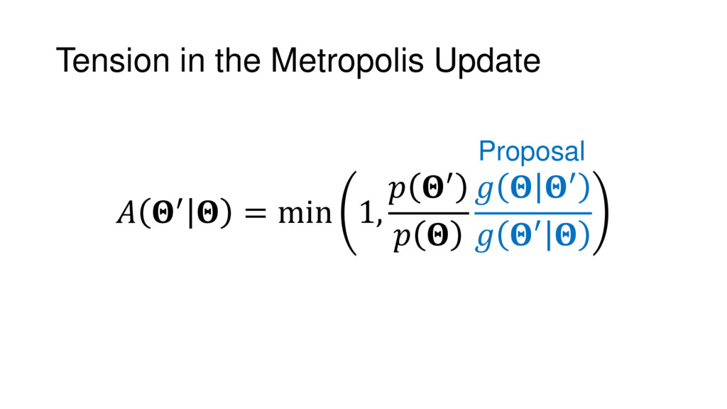
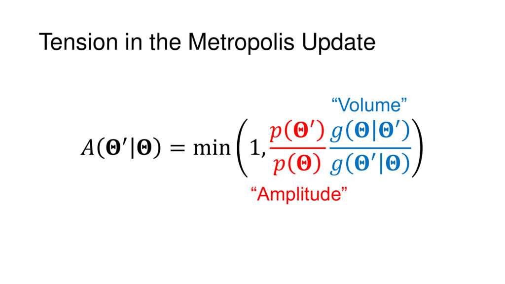
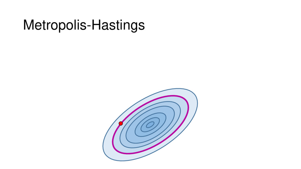
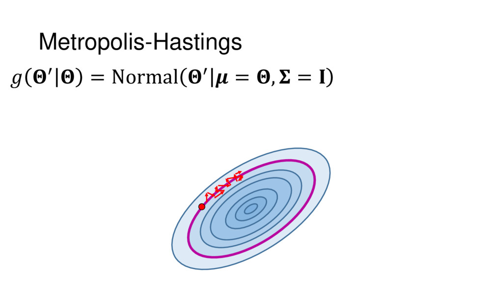
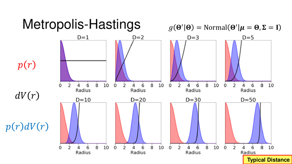
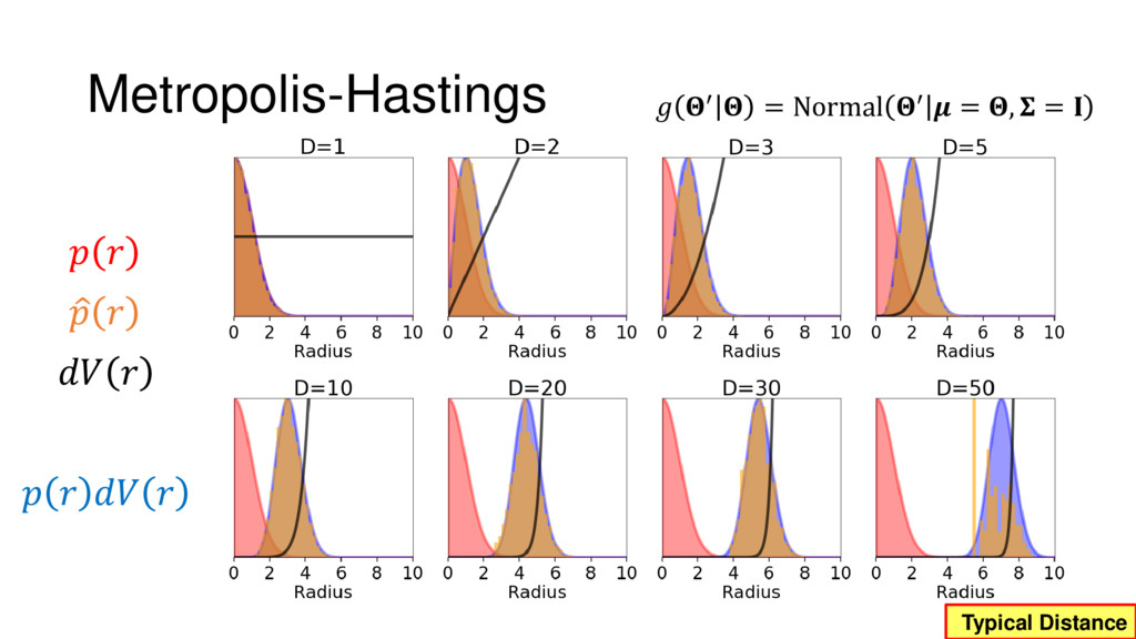
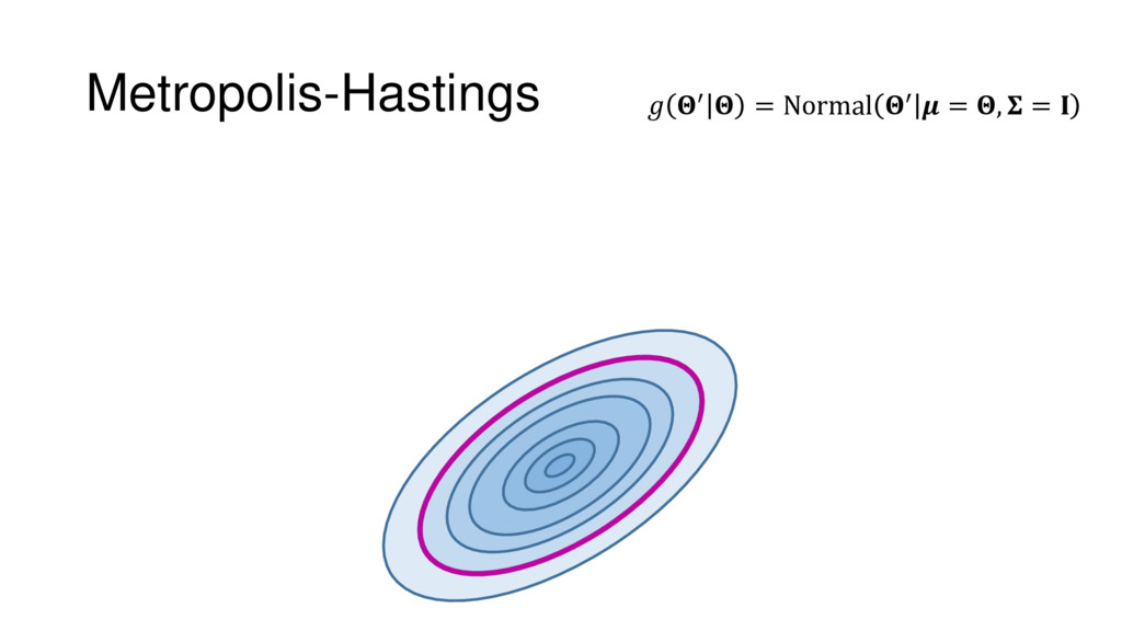
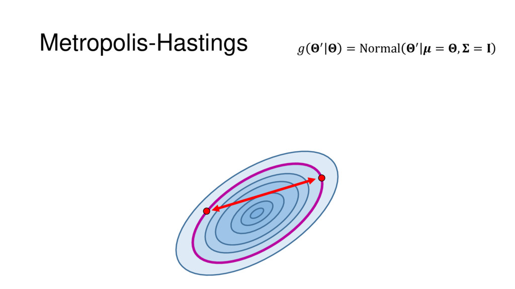
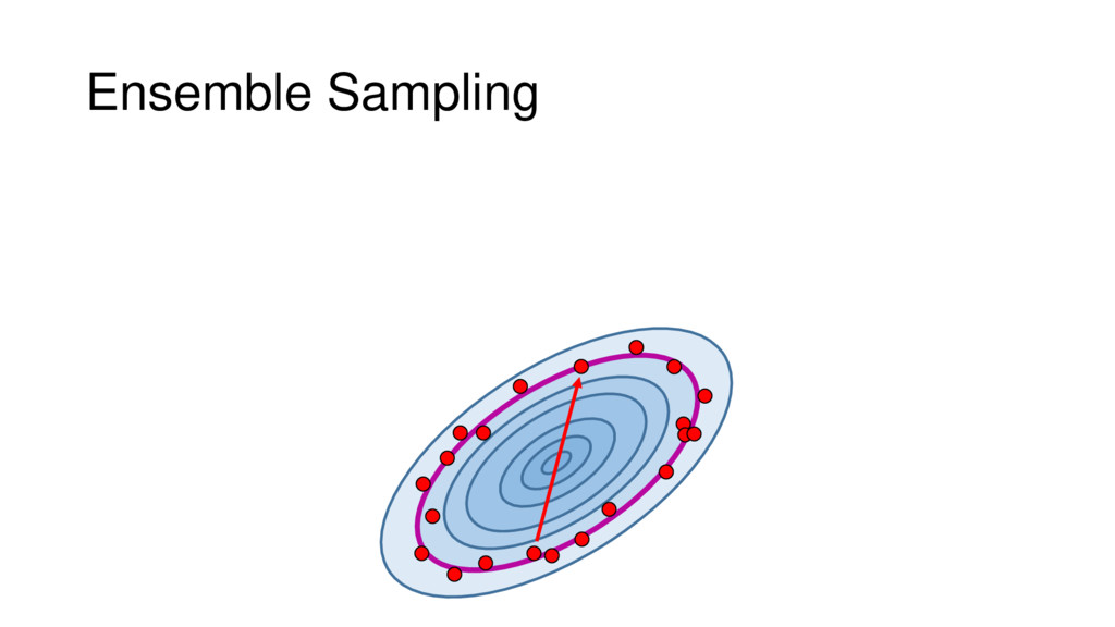
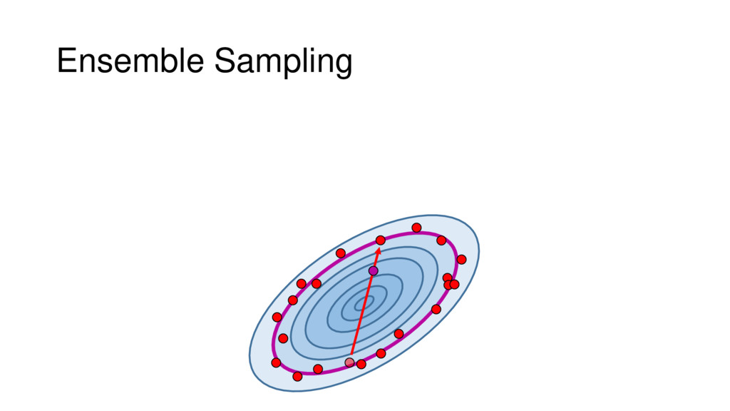
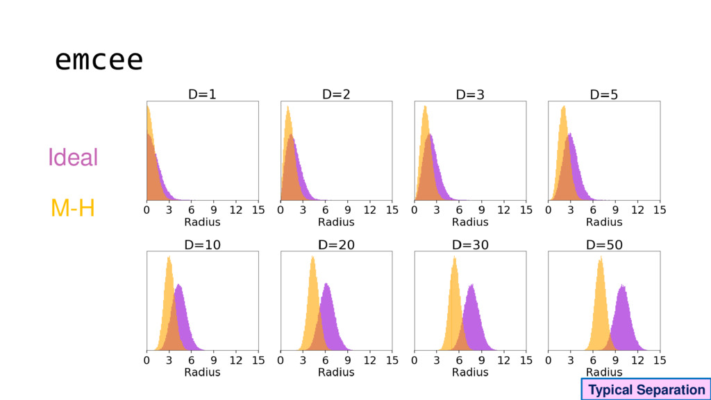
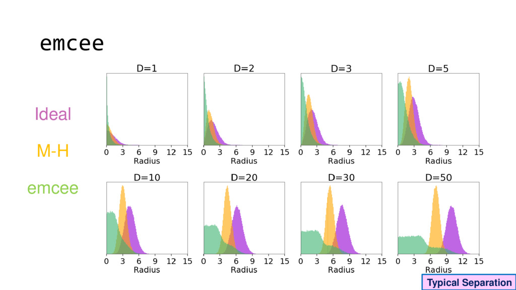
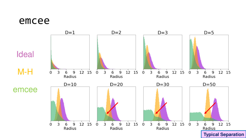
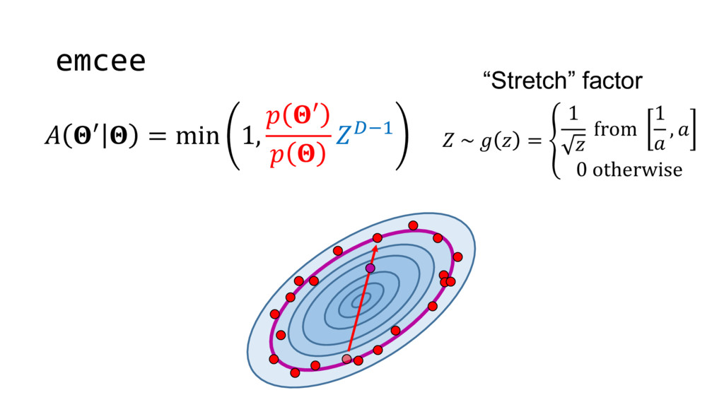
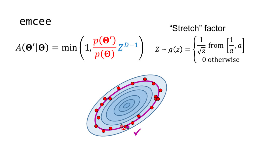
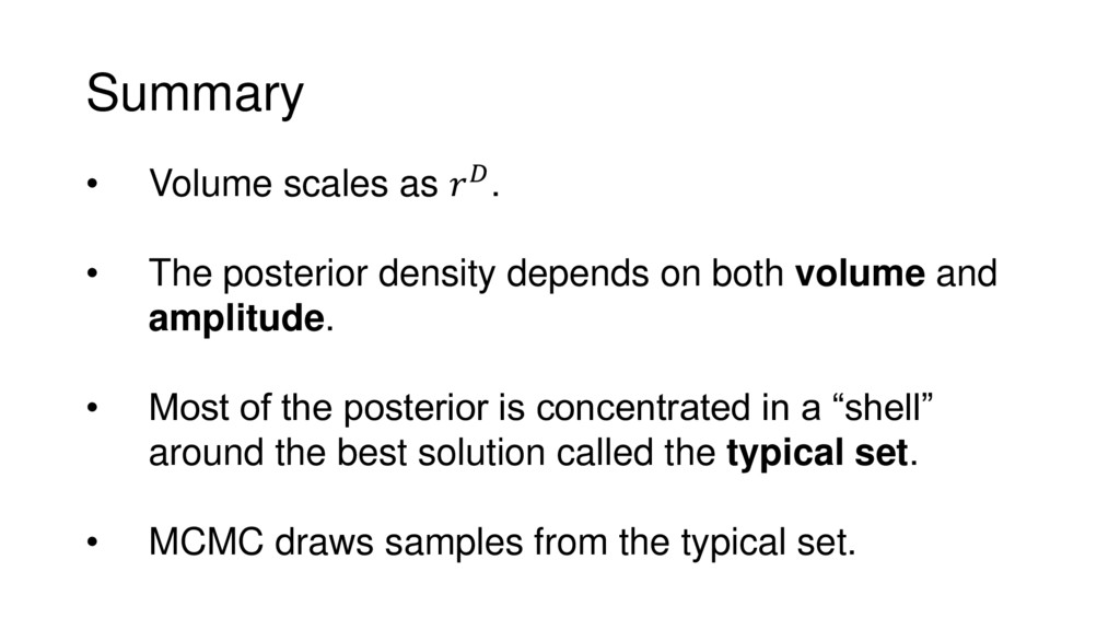
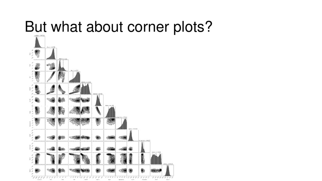
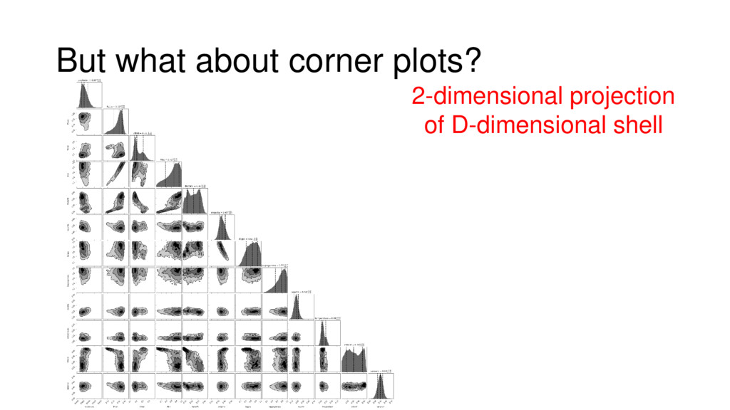
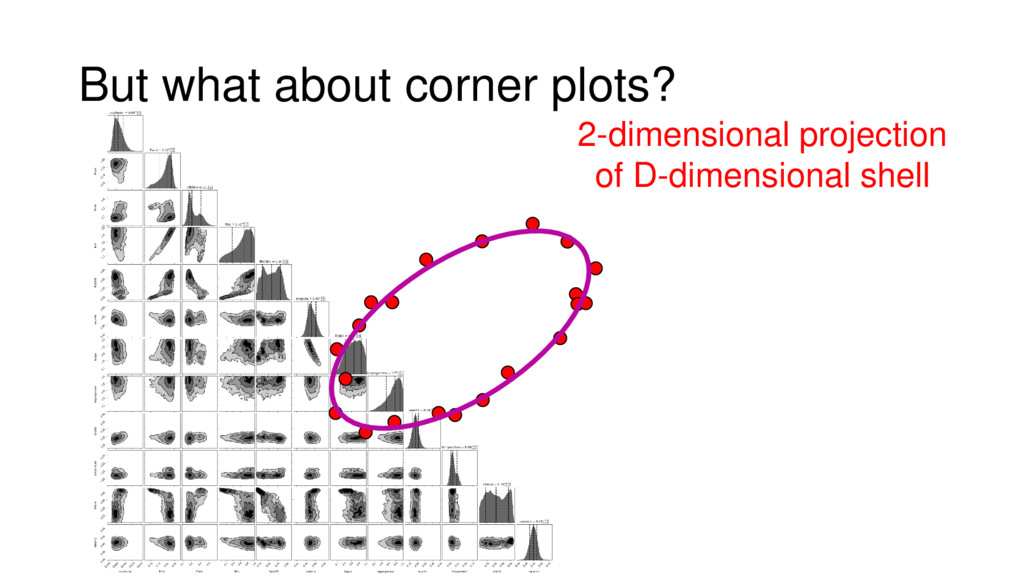
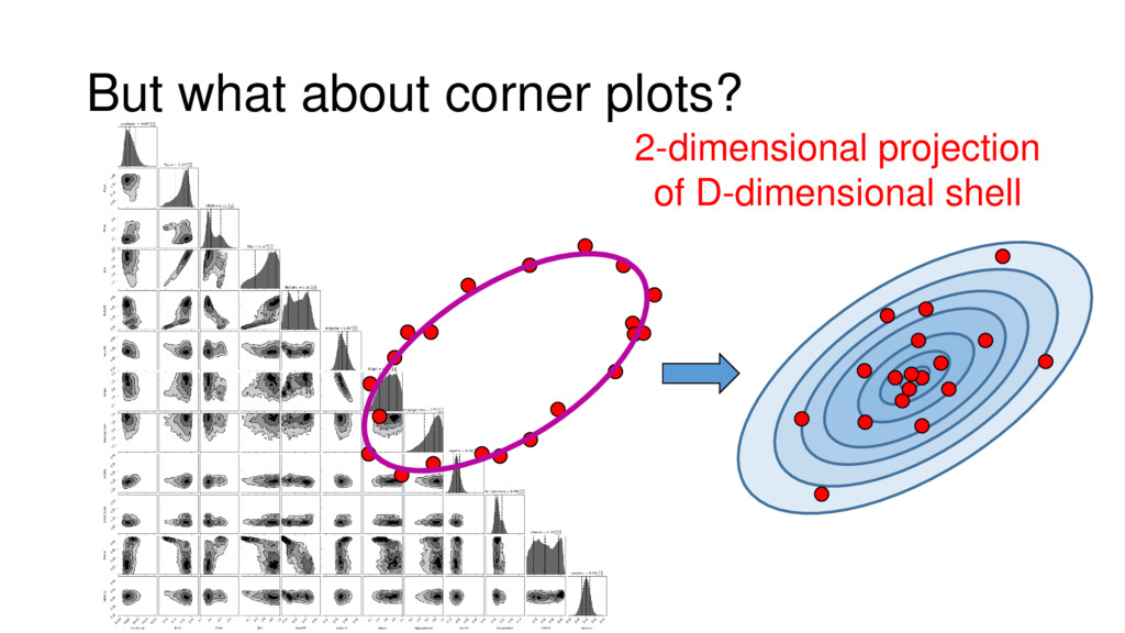
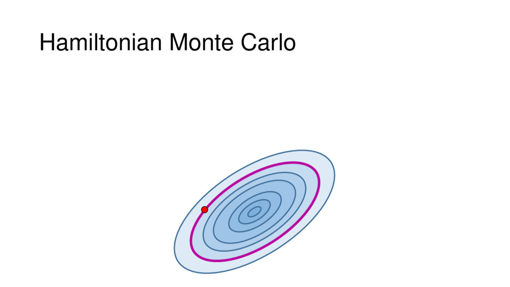
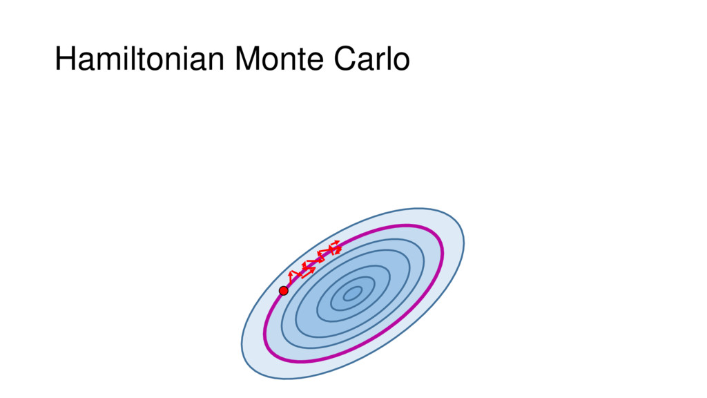
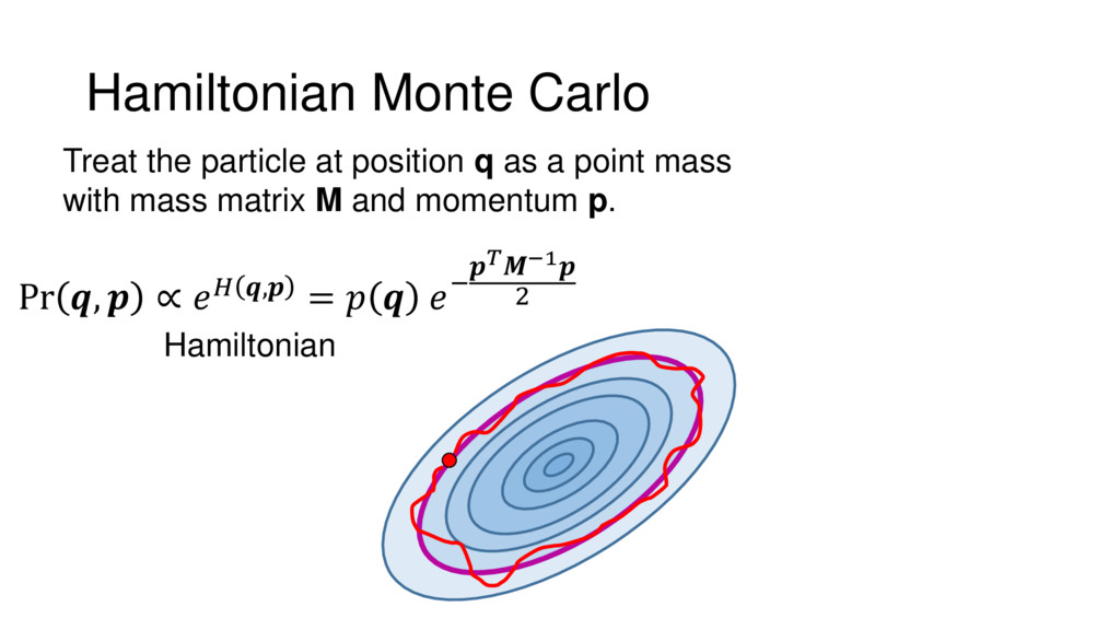
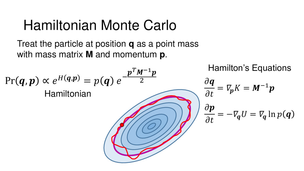
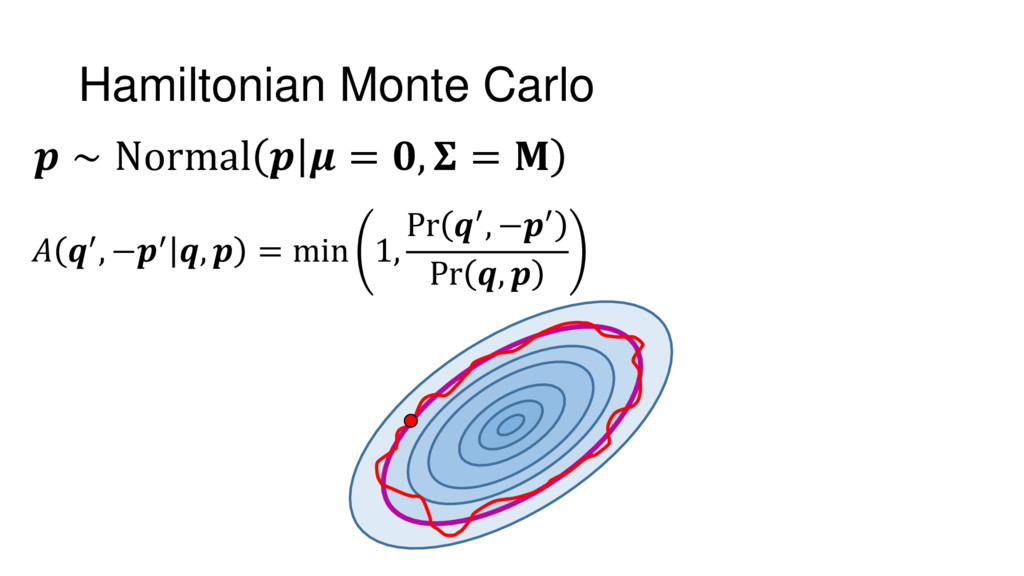
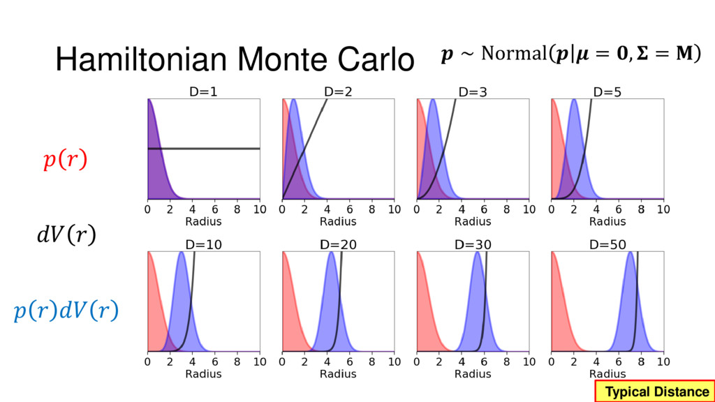
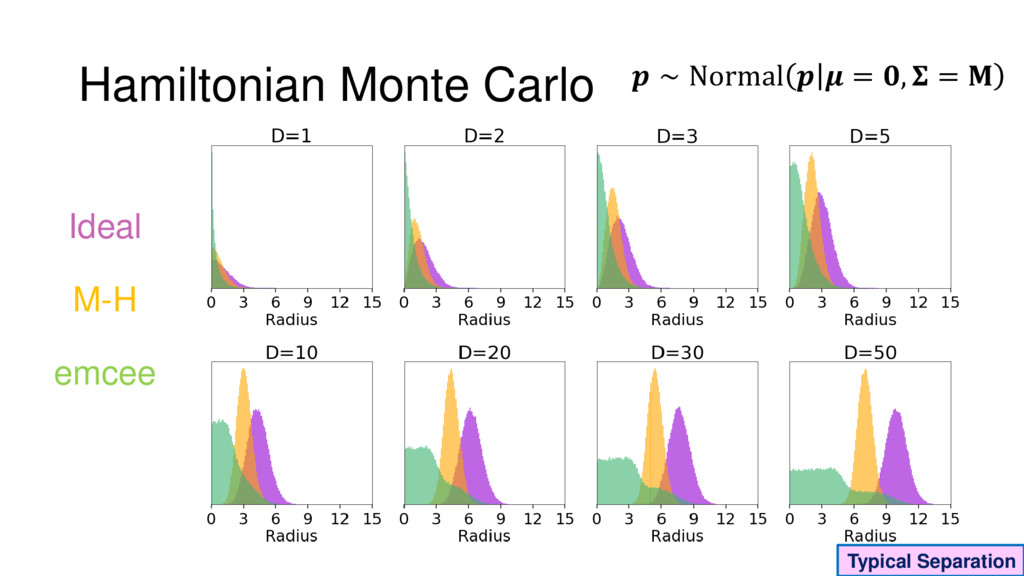
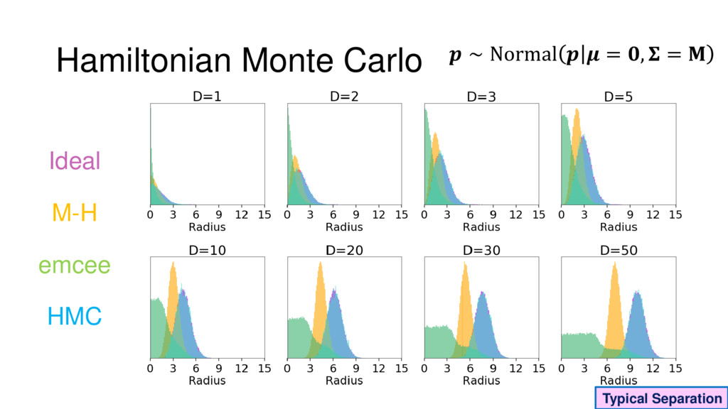
Although typical sets are important in understanding how/why sampling algorithms (do not) work, they are rarely taught when most astronomers are introduced to sampling methods such as Markov Chain Monte Carlo (MCMC). I introduce the idea of typical sets using some basic examples and show why they make sampling difficult in higher dimensions. I then outline how their behavior shapes various MCMC algorithms such as (Adaptive) Metropolis-Hastings, ensemble sampling, and Hamiltonian Monte Carlo. See https://github.com/joshspeagle/typical_sets for additional resources.

Transcript

1. Typical Sets:
   What They Are and How
   to (Hopefully) Find Them
   Josh Speagle
   jspeagle@cfa.harvard.edu
   Based on this talk by Michael Betancourt at StanCon.
   

   View Slide

2. Intended Audience
   • Some experience with the basics of Bayesian statistics.
   

   View Slide

3. Intended Audience
   • Some experience with the basics of Bayesian statistics.
   • Some experience using MCMC for research.
   

   View Slide

4. Intended Audience
   • Some experience with the basics of Bayesian statistics.
   • Some experience using MCMC for research.
   • Have heard of ensemble sampling methods such as
   emcee.
   

   View Slide

5. Bayesian Inference
   

   View Slide

6. Bayesian Inference
   Pr , M =
   Pr , M Pr |M
   Pr M
   Bayes’ Theorem
   

   View Slide

7. Bayesian Inference
   Pr , M =
   Pr , M Pr |M
   Pr M
   Bayes’ Theorem
   Parameters
   

   View Slide

8. Bayesian Inference
   Pr , M =
   Pr , M Pr |M
   Pr M
   Bayes’ Theorem
   Data
   Parameters
   

   View Slide

9. Bayesian Inference
   Pr , M =
   Pr , M Pr |M
   Pr M
   Bayes’ Theorem
   Data
   Parameters
   Model
   

   View Slide

10. Bayesian Inference
    Pr , M =
    Pr , M Pr |M
    Pr M
    Bayes’ Theorem
    

    View Slide

11. Bayesian Inference
    Pr , M =
    Pr , M Pr |M
    Pr M
    Bayes’ Theorem
    Prior
    

    View Slide

12. Bayesian Inference
    Pr , M =
    Pr , M Pr |M
    Pr M
    Bayes’ Theorem
    Prior
    Likelihood
    

    View Slide

13. Bayesian Inference
    Pr , M =
    Pr , M Pr |M
    Pr M
    Bayes’ Theorem
    Prior
    Likelihood
    Posterior
    

    View Slide

14. Bayesian Inference
    Pr , M =
    Pr , M Pr |M
    Pr M
    Bayes’ Theorem
    Prior
    Likelihood
    Posterior
    Evidence
    

    View Slide

15. Bayesian Inference
    =
    ℒ
    
    Bayes’ Theorem
    ≡
    Ω
    ℒ
    Posterior
    Likelihood Prior
    Evidence
    

    View Slide

16. Bayesian Inference
    =
    ℒ
    
    Bayes’ Theorem
    Posterior
    Likelihood Prior
    Evidence ≡
    Ω
    ℒ
    

    View Slide

17. Where is the posterior?
    ≡
    Ω
    
    

    View Slide

18. Where is the posterior?
    ≡
    {: =}
    
    

    View Slide

19. Where is the posterior?
    ≡
    0
    ∞
    
    

    View Slide

20. Where is the posterior?
    ≡
    0
    ∞
    
    
    =
    
    

    View Slide

21. Where is the posterior?
    ≡
    0
    ∞
    
    “Amplitude”
    “Volume”
    
    =
    
    

    View Slide

22. 
    =
    
    Where is the posterior?
    ≡
    0
    ∞
    
    “Typical Set”
    

    View Slide

23. Typical Sets: Gaussian Example
    

    View Slide

24. Typical Sets: Gaussian Example
    ∝
    0
    ∞
    −
    2
    2
    

    View Slide

25. Typical Sets: Gaussian Example
    ∝
    0
    ∞
    −
    2
    2 ∝
    0
    ∞
    −
    2
    2 −1
    

    View Slide

26. Typical Distance
    Typical Sets: Gaussian Example
    
    
    
    

    View Slide

27. 
    =
    
    Where is the posterior?
    ≡
    0
    ∞
    
    “Typical Set”
    

    View Slide

28. 
    =
    
    Where is the posterior?
    ≡
    0
    ∞
    
    “Typical Set”
    

    View Slide

29. 
    =
    
    Where is the posterior?
    ≡
    0
    ∞
    
    “Typical Set”
    

    View Slide

30. 
    =
    
    Where is the posterior?
    ≡
    0
    ∞
    
    “Typical Set”
    MCMC wants to draw
    samples from this “shell”
    

    View Slide

31. Tension in the Metropolis Update
    ′ = min 1,
    ′
    
    ′
    ′
    

    View Slide

32. Tension in the Metropolis Update
    ′ = min 1,
    ′
    
    ′
    ′
    Proposal
    

    View Slide

33. Tension in the Metropolis Update
    ′ = min 1,
    ′
    
    ′
    ′
    “Volume”
    

    View Slide

34. Tension in the Metropolis Update
    ′ = min 1,
    ′
    
    ′
    ′
    “Volume”
    “Amplitude”
    

    View Slide

35. Metropolis-Hastings
    

    View Slide

36. Metropolis-Hastings
    ′ = Normal ′ = , =
    

    View Slide

37. 
    
    
    Metropolis-Hastings ′ = Normal ′ = , =
    Typical Distance
    

    View Slide

38. Metropolis-Hastings ′ = Normal ′ = , =
    
    
    
    
    Typical Distance
    

    View Slide

39. Metropolis-Hastings ′ = Normal ′ = , =
    

    View Slide

40. Metropolis-Hastings ′ = Normal ′ = , =
    

    View Slide

41. Ideal
    Metropolis-Hastings ′ = Normal ′ = , =
    Typical Separation
    

    View Slide

42. Ideal
    Metropolis-Hastings ′ = Normal ′ = , =
    Typical Separation
    M-H
    

    View Slide

43. Ideal
    Metropolis-Hastings ′ = Normal ′ = , = s
    Typical Separation
    Adaptive
    M-H
    

    View Slide

44. Ensemble Sampling
    

    View Slide

45. Ensemble Sampling
    

    View Slide

46. Ensemble Sampling
    

    View Slide

47. Ensemble Sampling
    

    View Slide

48. Ensemble Sampling
    

    View Slide

49. Ensemble Sampling
    

    View Slide

50. emcee
    ′ = min 1,
    ′
    
    −1
    ~ =
    1
    
    from
    1
    
    ,
    0 otherwise
    “Stretch” factor
    

    View Slide

51. Ideal
    Typical Separation
    emcee
    M-H
    

    View Slide

52. Ideal
    Typical Separation
    emcee
    M-H
    emcee
    

    View Slide

53. Ideal
    Typical Separation
    emcee
    M-H
    emcee
    

    View Slide

54. Ideal
    Typical Separation
    emcee
    M-H
    emcee
    After weighting by
    acceptance probability
    

    View Slide

55. emcee
    ′ = min 1,
    ′
    
    −1
    ~ =
    1
    
    from
    1
    
    ,
    0 otherwise
    “Stretch” factor
    

    View Slide

56. emcee
    ′ = min 1,
    ′
    
    −1
    ~ =
    1
    
    from
    1
    
    ,
    0 otherwise
    “Stretch” factor
    
    

    View Slide

57. Summary
    • Volume scales as .
    • The posterior density depends on both volume and
    amplitude.
    • Most of the posterior is concentrated in a “shell”
    around the best solution called the typical set.
    • MCMC draws samples from the typical set.
    

    View Slide

58. But what about corner plots?
    

    View Slide

59. But what about corner plots?
    2-dimensional projection
    of D-dimensional shell
    

    View Slide

60. But what about corner plots?
    2-dimensional projection
    of D-dimensional shell
    

    View Slide

61. But what about corner plots?
    2-dimensional projection
    of D-dimensional shell
    

    View Slide

62. Hamiltonian Monte Carlo
    

    View Slide

63. Hamiltonian Monte Carlo
    

    View Slide

64. Hamiltonian Monte Carlo
    

    View Slide

65. Hamiltonian Monte Carlo
    Treat the particle at position q as a point mass
    with mass matrix M and momentum p.
    Pr , ∝ , = −
    −1
    2
    Hamiltonian
    

    View Slide

66. Hamiltonian Monte Carlo
    Pr , ∝ , = −
    −1
    2
    Treat the particle at position q as a point mass
    with mass matrix M and momentum p.
    
    
    =
    = −1
    
    
    = −
    =
    ln
    Hamiltonian
    Hamilton’s Equations
    

    View Slide

67. Hamiltonian Monte Carlo
    ′, −′ , = min 1,
    Pr ′, −′
    Pr ,
    ∼ Normal = , =
    

    View Slide

68. Typical Distance
    Hamiltonian Monte Carlo
    
    
    
    ∼ Normal = , =
    

    View Slide

69. Typical Distance
    Hamiltonian Monte Carlo
    
    
    
    
    ∼ Normal = , =
    

    View Slide

70. Ideal
    Typical Separation
    M-H
    emcee
    Hamiltonian Monte Carlo ∼ Normal = , =
    

    View Slide

71. Ideal
    Typical Separation
    M-H
    emcee
    Hamiltonian Monte Carlo ∼ Normal = , =
    HMC
    

    View Slide