An Introduction to (Dynamic) Nested Sampling

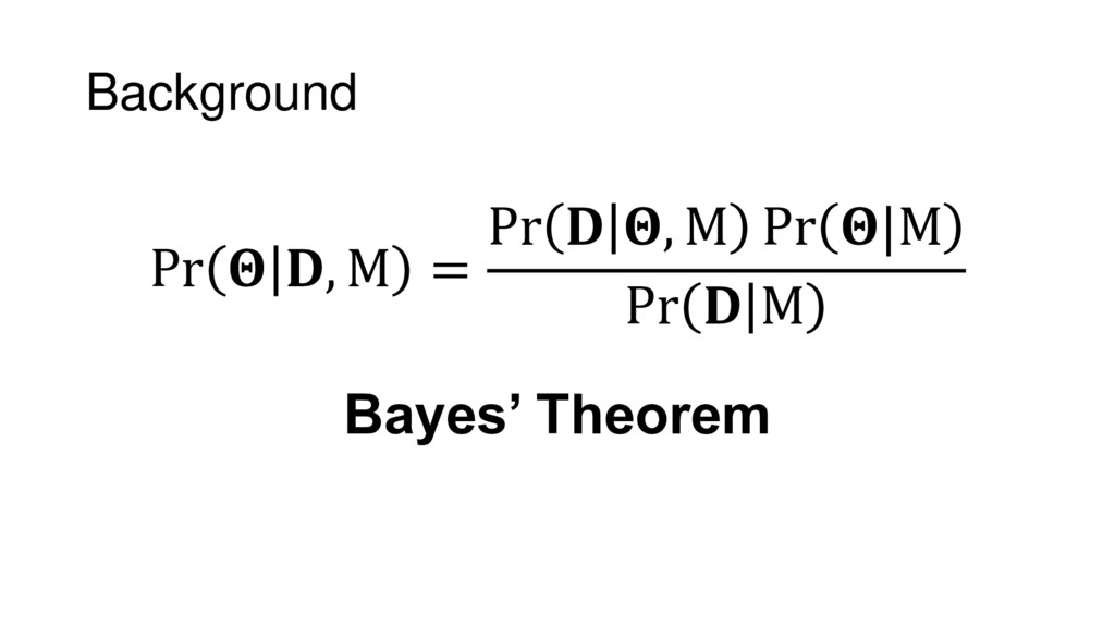
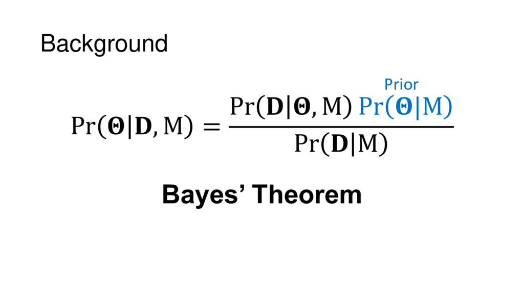
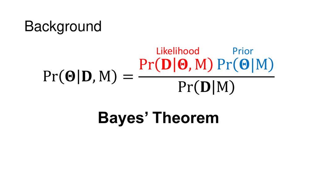
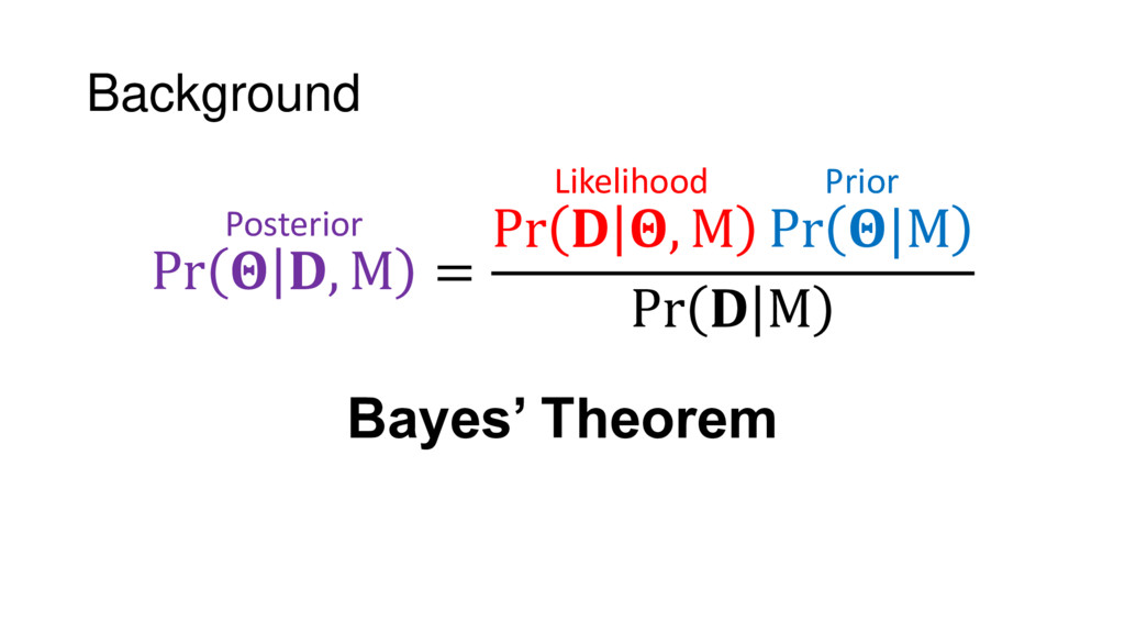
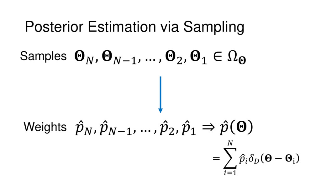
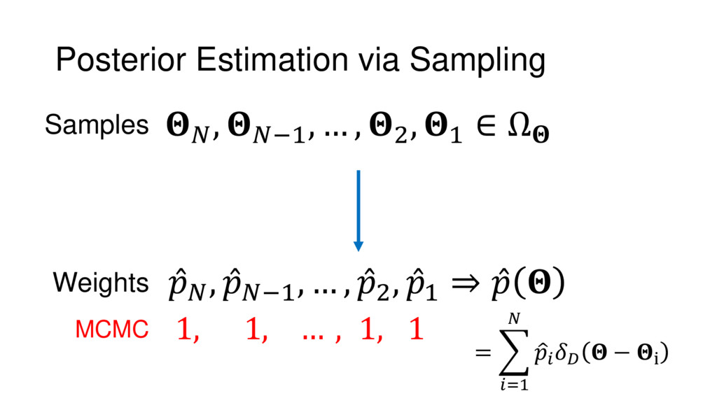
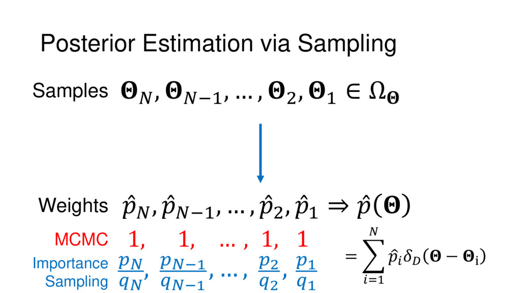
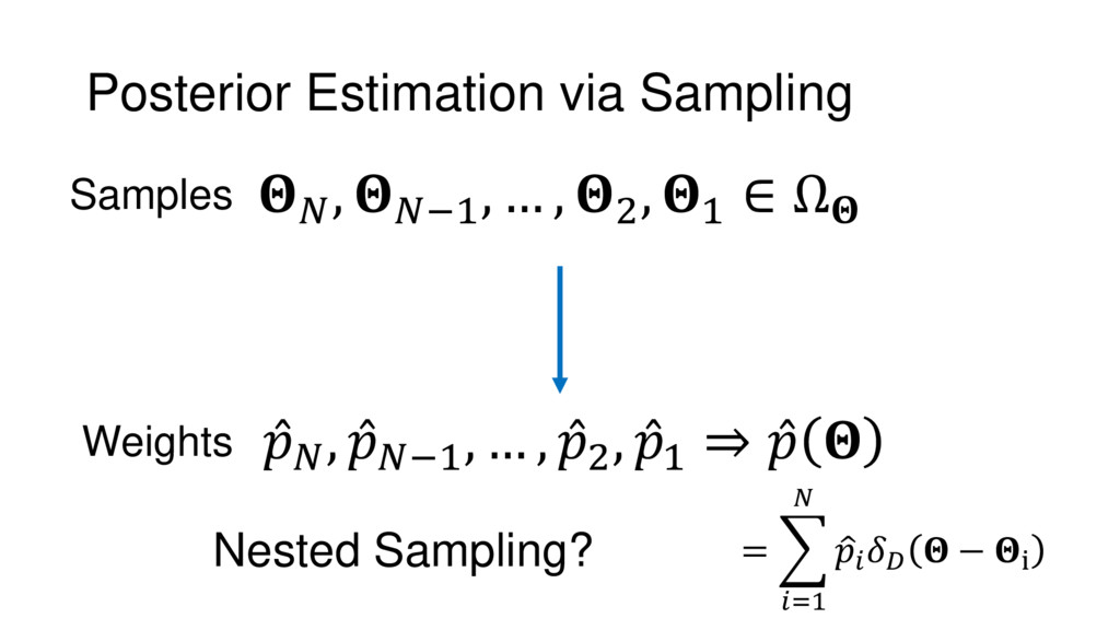
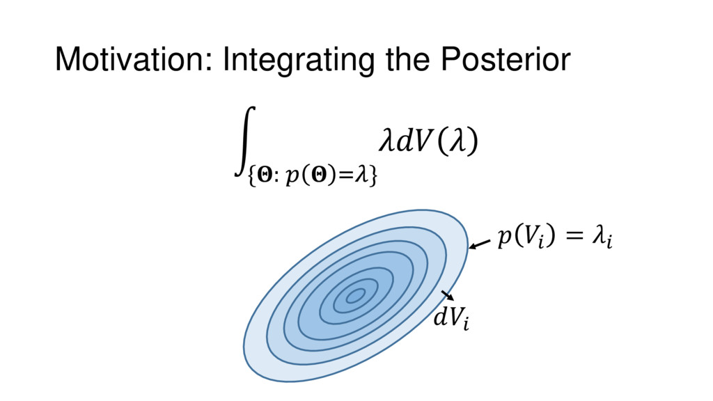
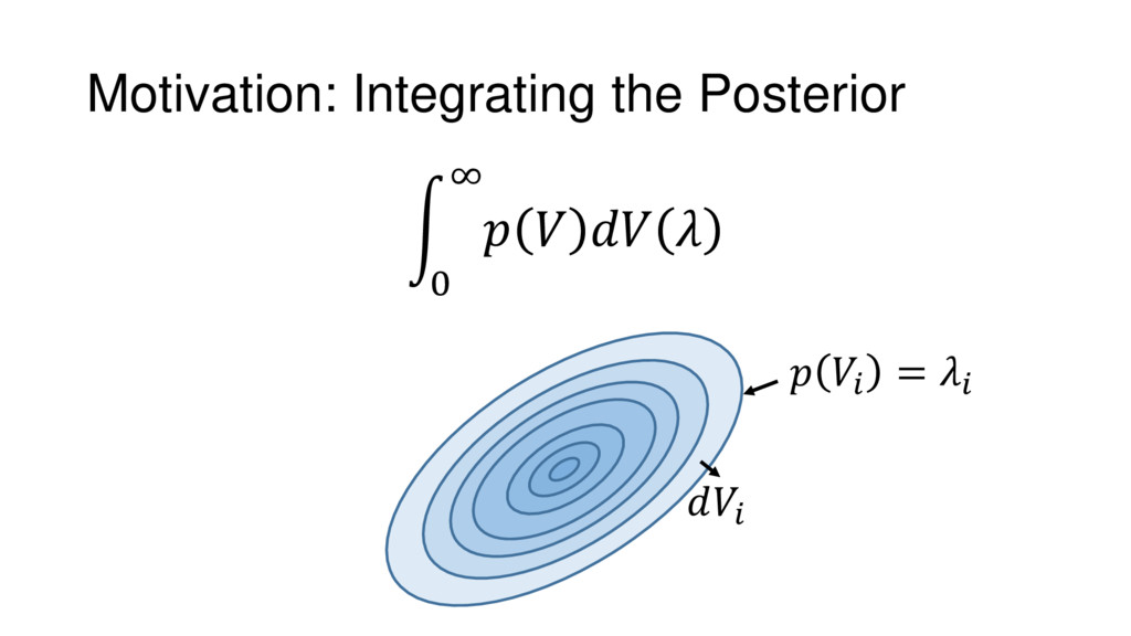
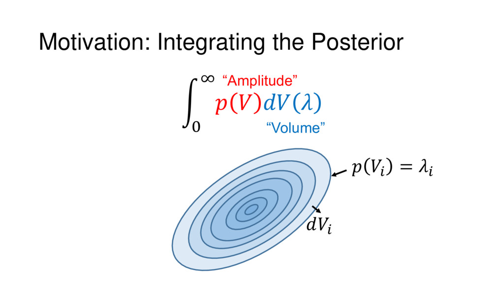
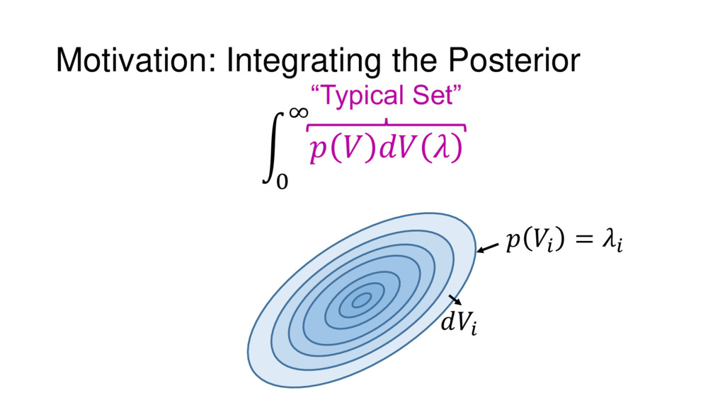
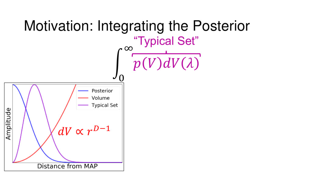
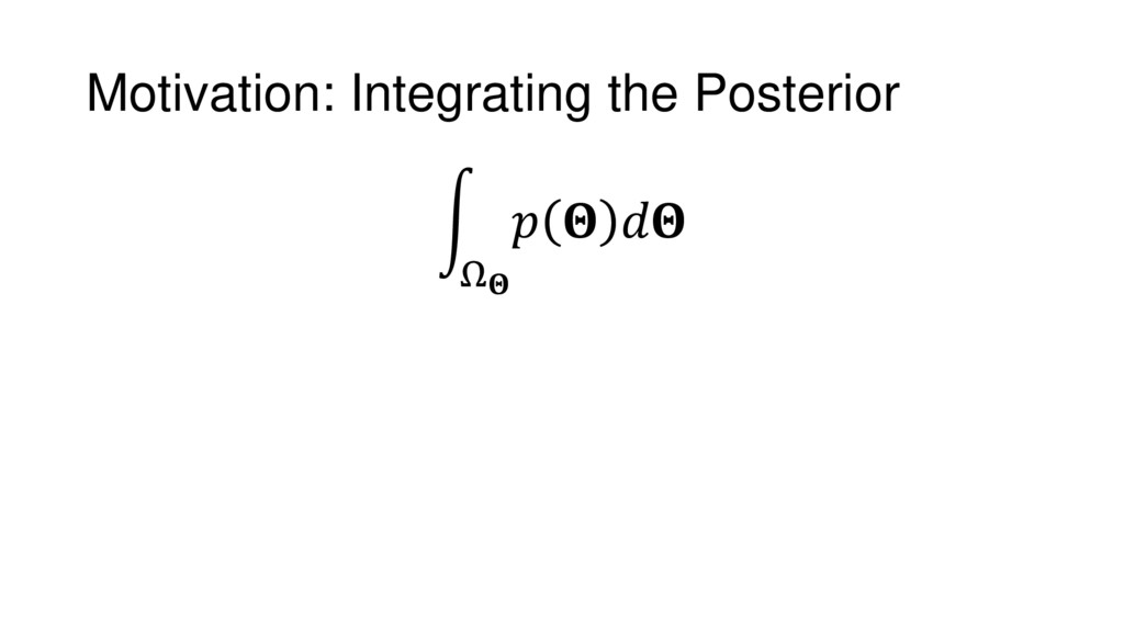
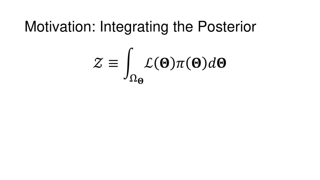
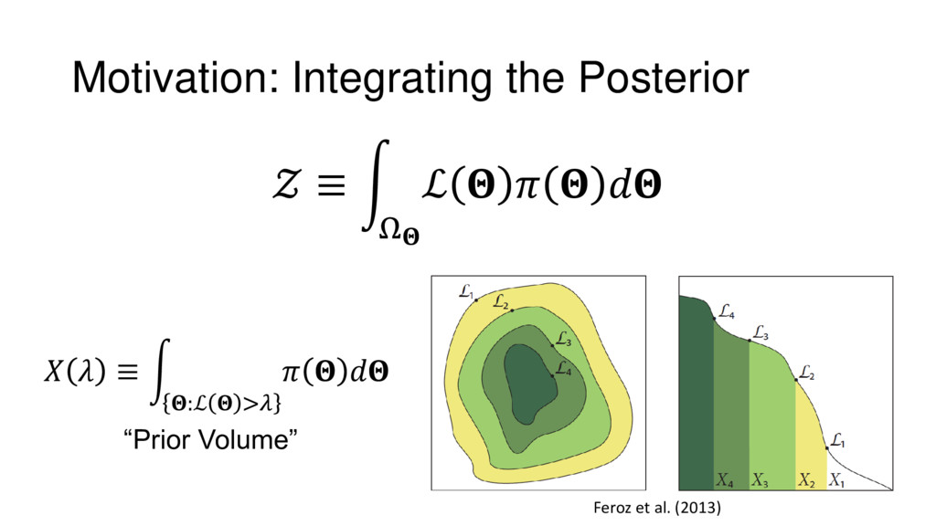
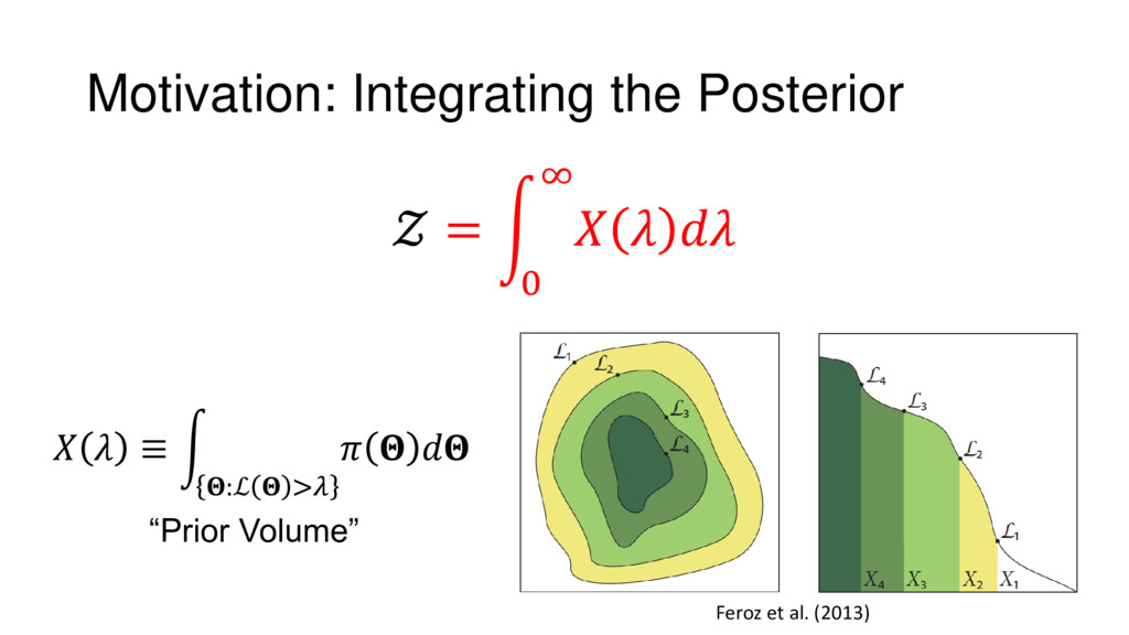
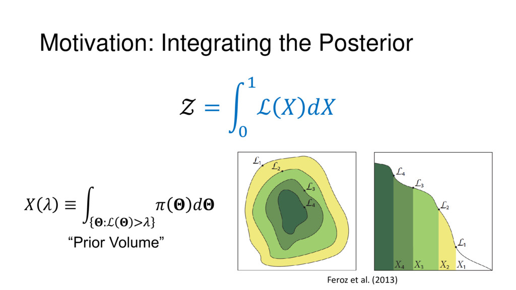
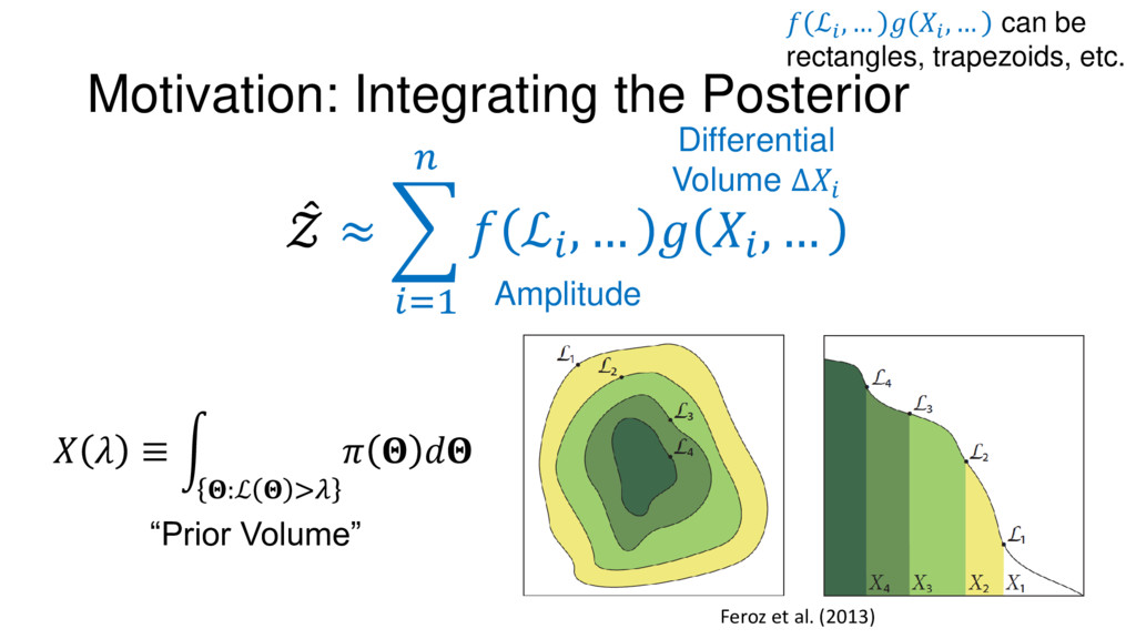
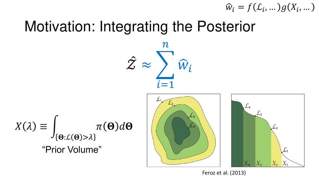
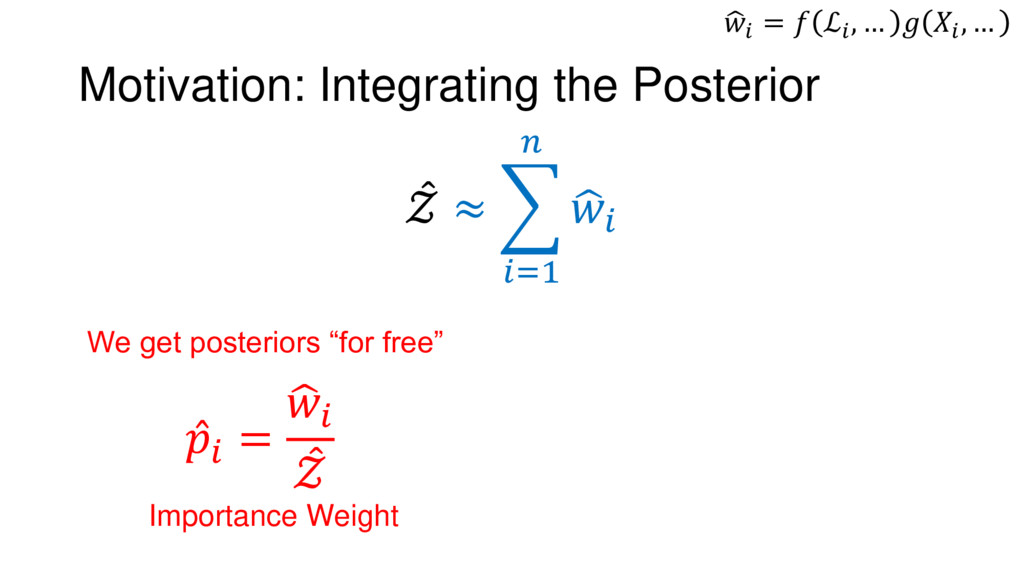
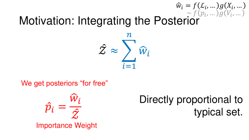
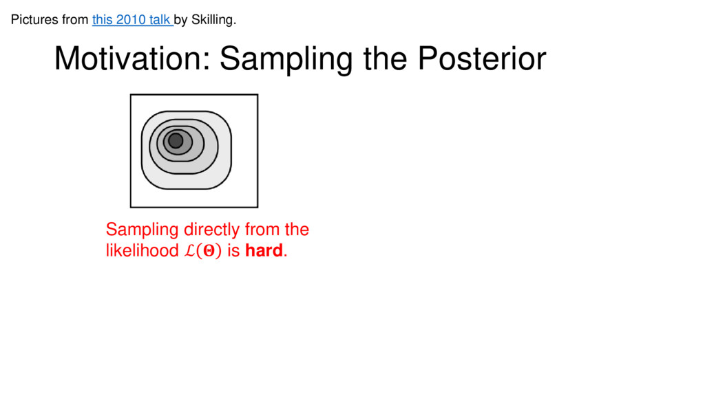
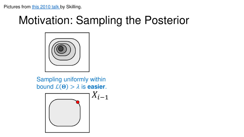
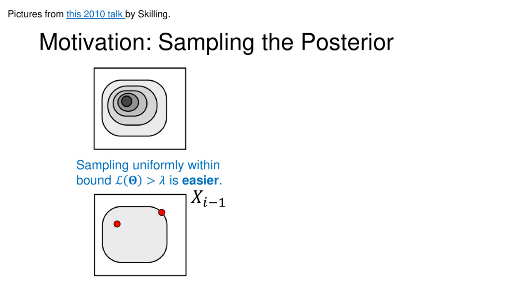
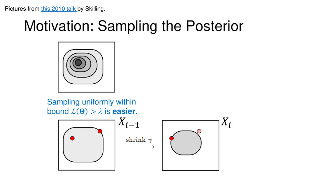
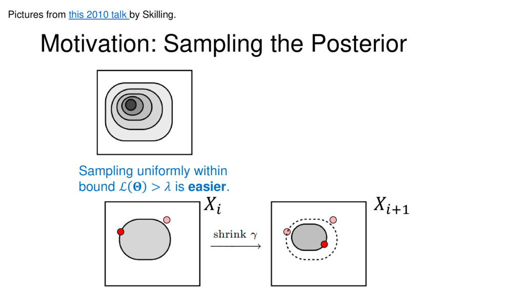
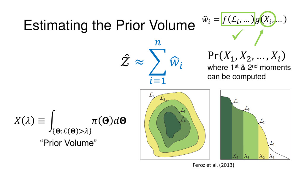
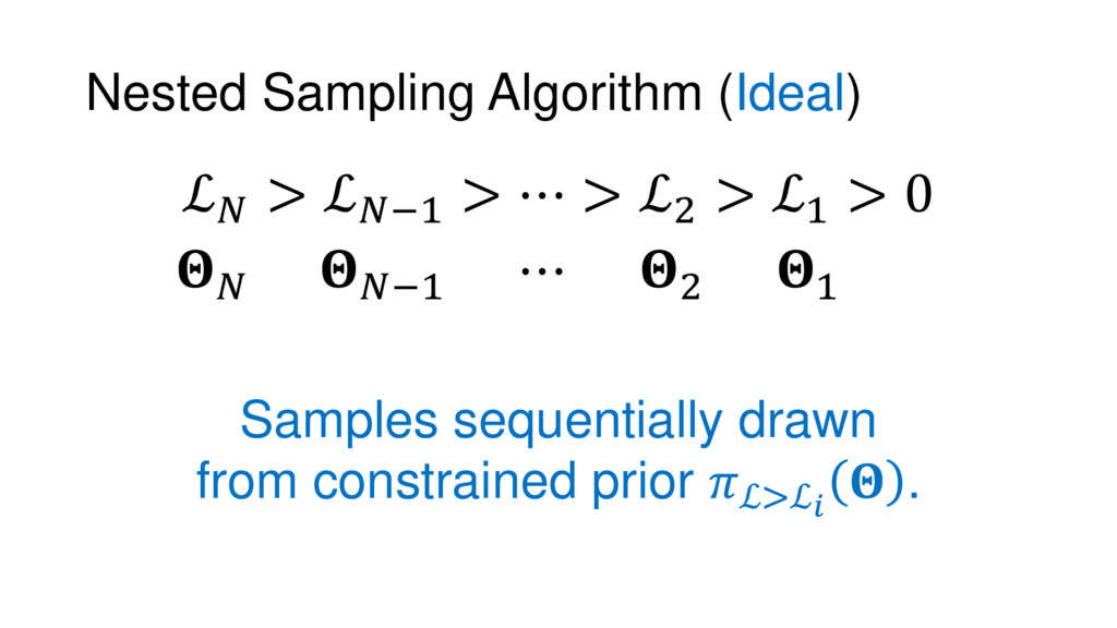
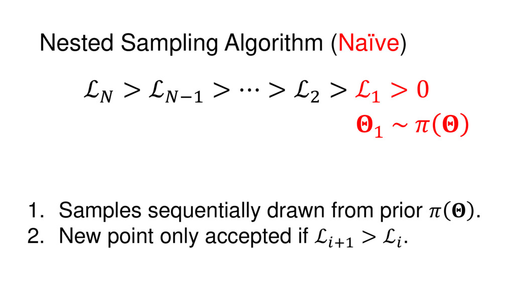
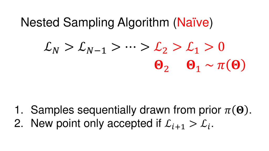
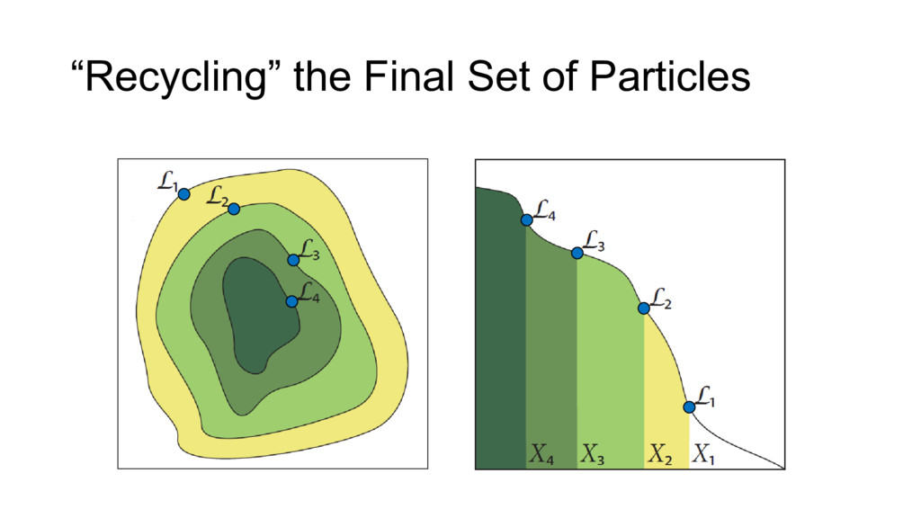
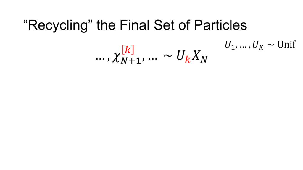
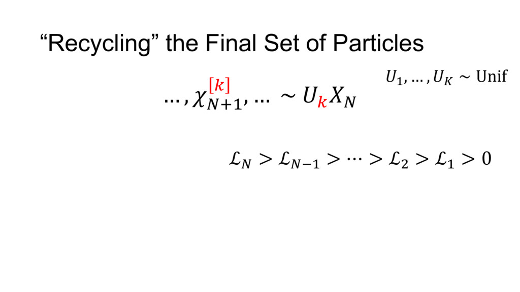
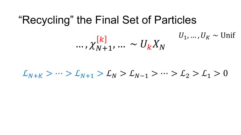
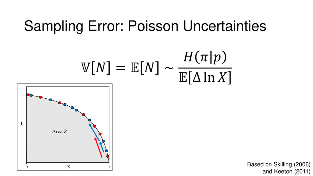
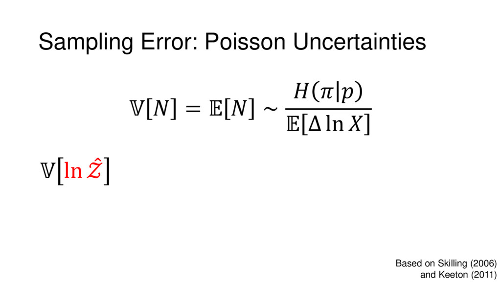
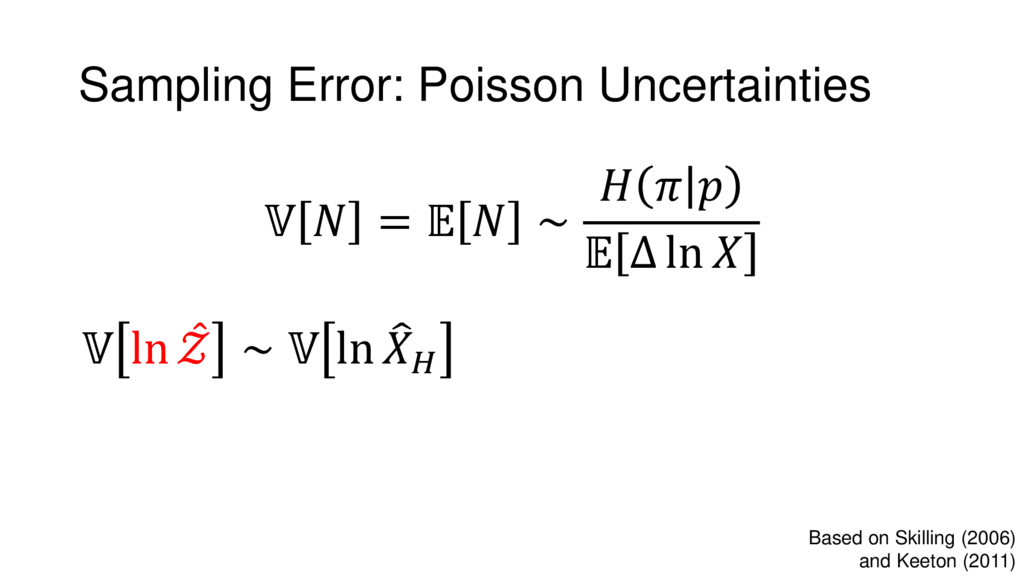
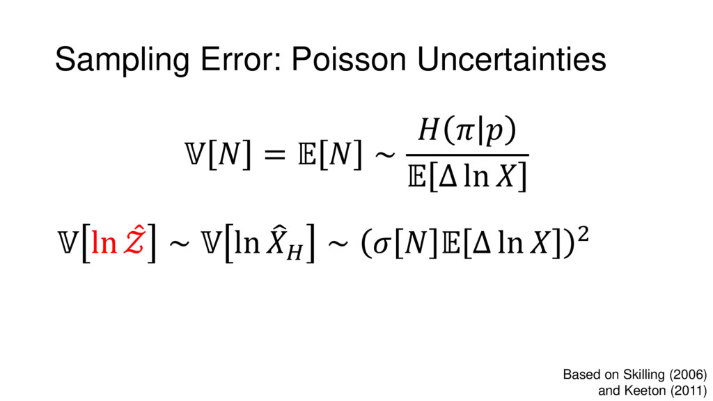
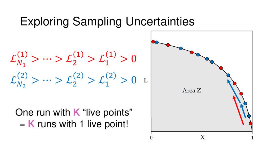
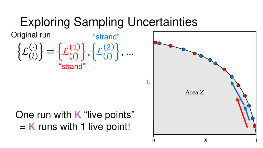
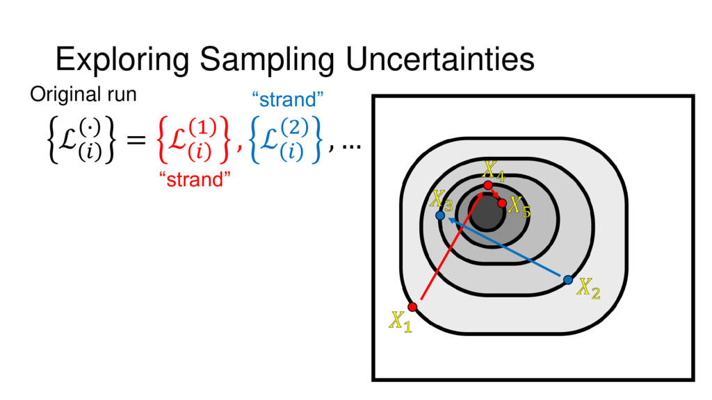
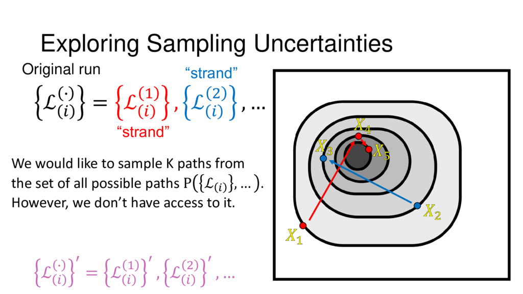
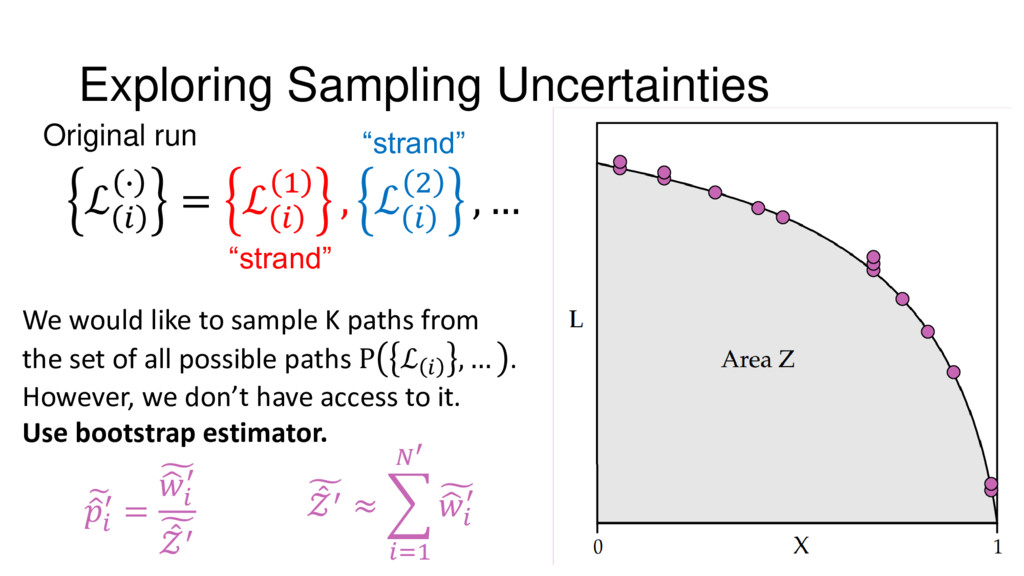
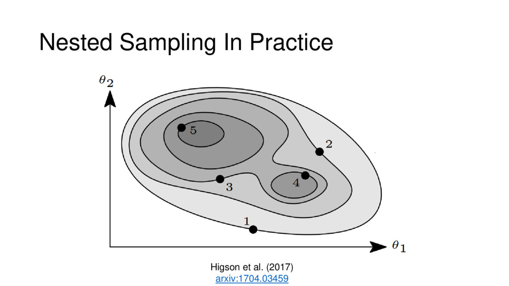
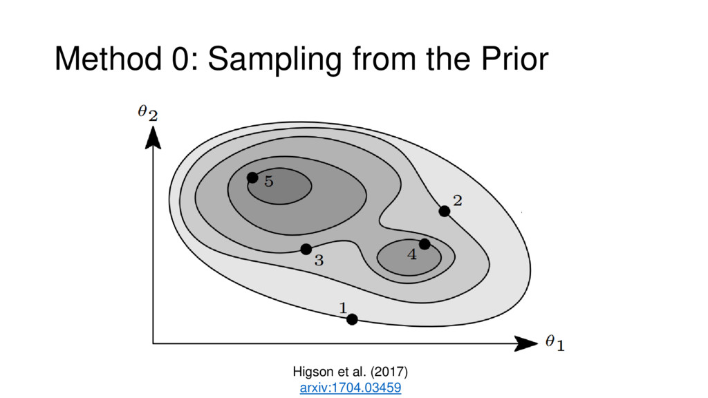
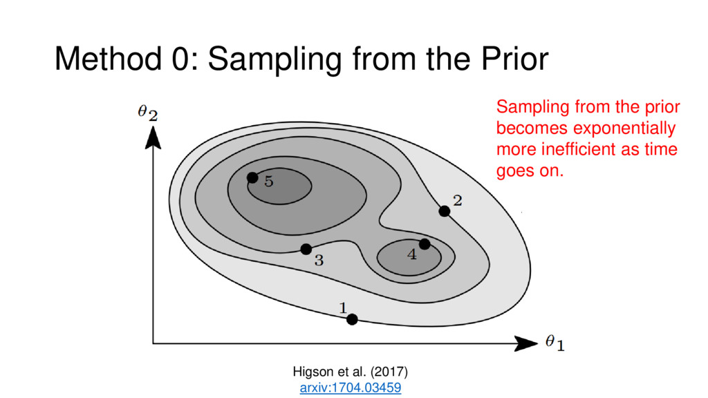
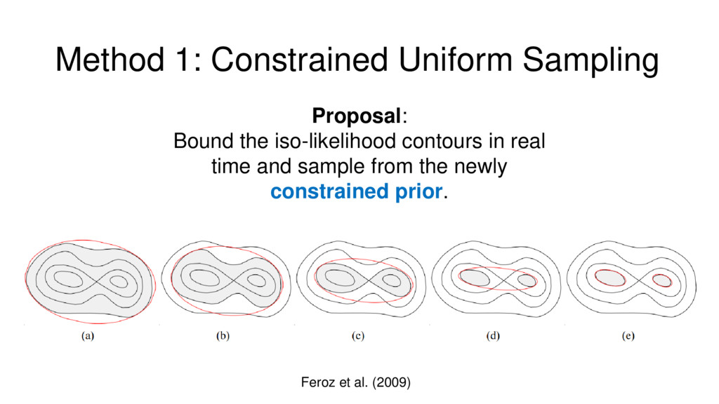
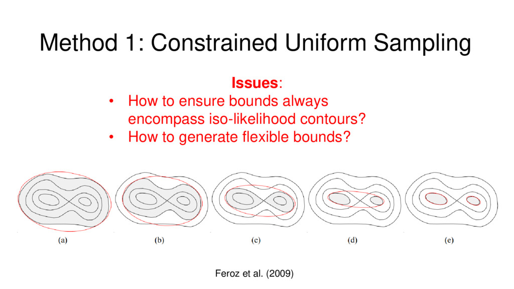
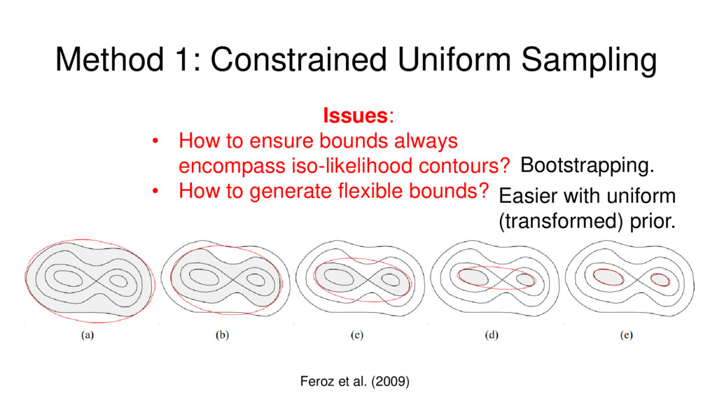
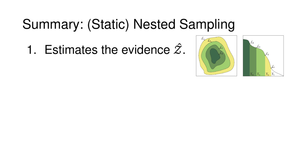
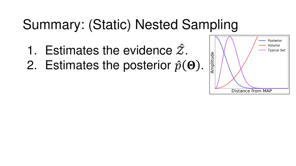
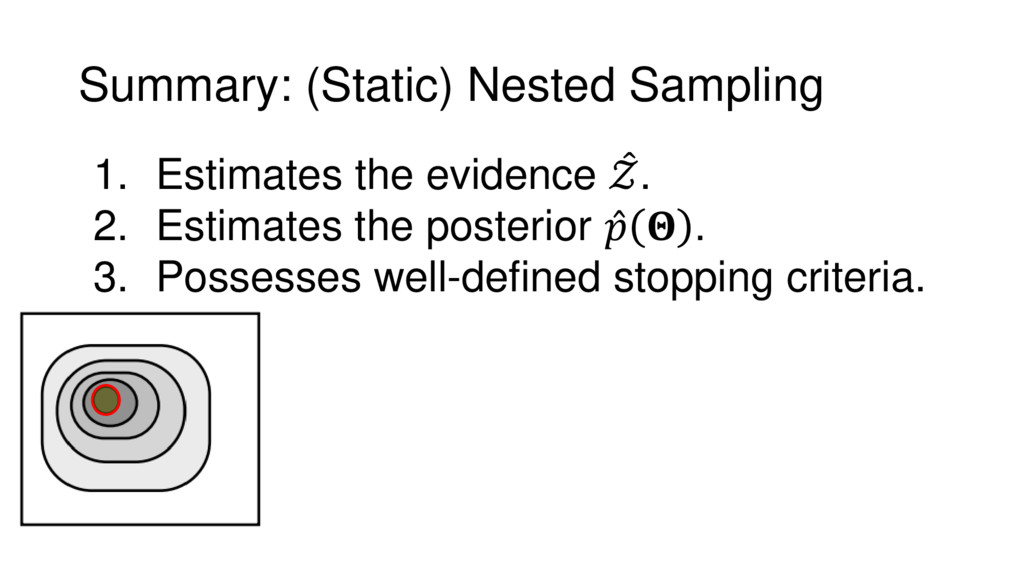
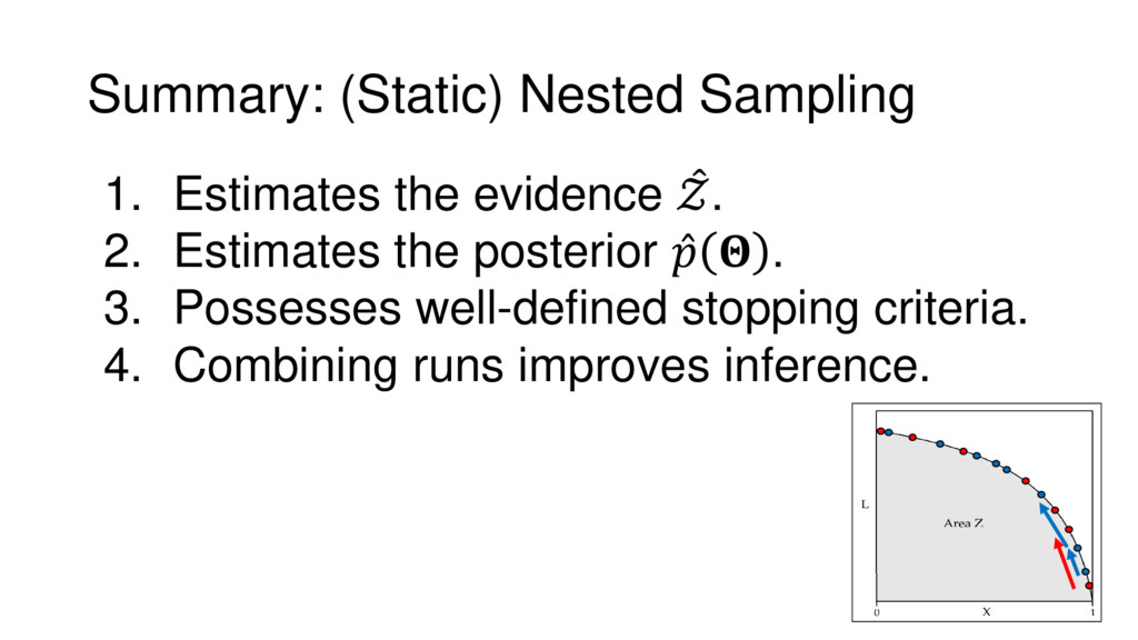
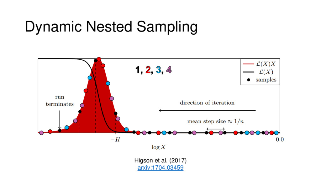
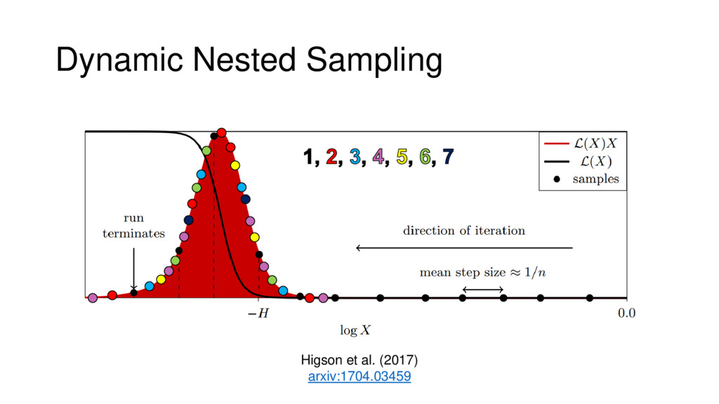
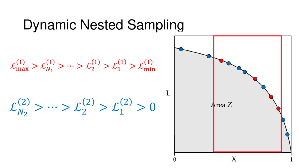
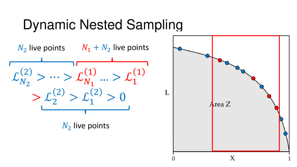
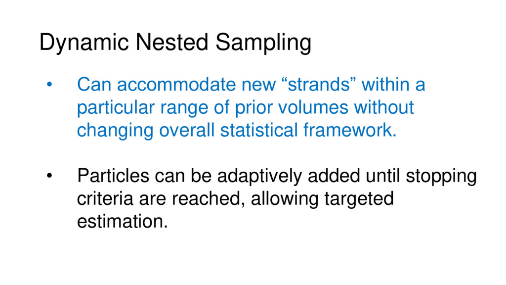
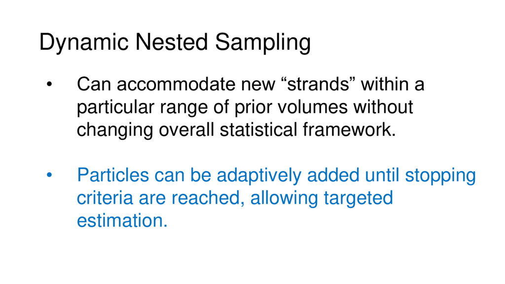
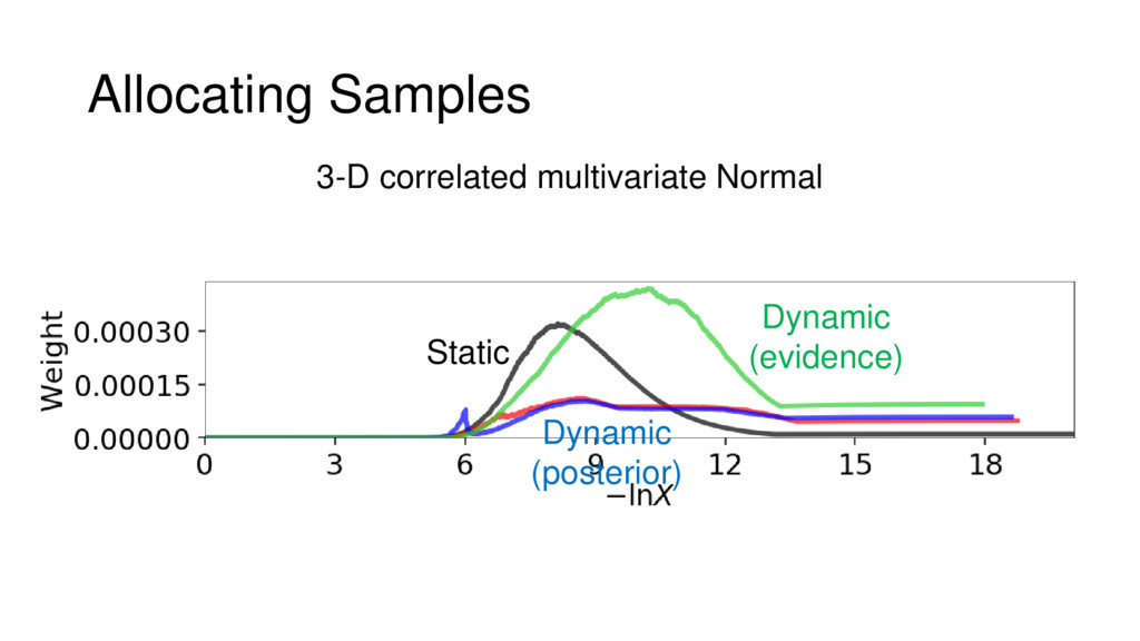
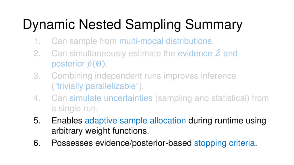
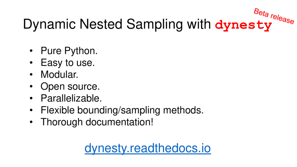
Nested Sampling is a relatively new method for estimating the Bayesian evidence (with the posterior estimated as a byproduct) that integrates over the posterior by sampling in nested "shells" of constant likelihood. Its ability to sample from complex, multi-modal distributions in a flexible yet efficient way combined with several available sampling packages has contributed to its growing popularity in (astro)physics. In this talk I outline the basic motivation and theory behind Nested Sampling, derive various statistical properties associated with the method, and discuss how it is applied in practice. I also talk about how the overall framework can be extended in Dynamic Nested Sampling to accommodate adding samples "dynamically" during the course of a run. These samples can be allocated to maximize arbitrary objective functions, allowing Dynamic Nested Sampling to function as a posterior-oriented sampling method such as MCMC but with the added benefit of well-defined stopping criteria. I end with an application of Dynamic Nested Sampling to a variety of synthetic and real-world problems using an open-source Python package I've been developing (https://github.com/joshspeagle/dynesty/).

Transcript

1. An Introduction to (Dynamic) Nested Sampling Josh Speagle jspeagle@cfa.harvard.edu
2. Introduction
3. Background Pr , M = Pr , M Pr |M Pr M Bayes’ Theorem
4. Background Pr , M = Pr , M Pr |M Pr M Bayes’ Theorem Prior
5. Background Pr , M = Pr , M Pr |M Pr M Bayes’ Theorem Prior Likelihood
6. Background Pr , M = Pr , M Pr |M Pr M Bayes’ Theorem Prior Likelihood Posterior
7. Background Pr , M = Pr , M Pr |M Pr M Bayes’ Theorem Prior Likelihood Posterior Evidence
8. Background = ℒ Bayes’ Theorem ≡ Ω ℒ Posterior Likelihood Prior Evidence
9. Background = ℒ Bayes’ Theorem ≡ Ω ℒ Posterior Likelihood Prior Evidence
10. Posterior Estimation via Sampling , −1 , … , 2 , 1 ∈ Ω Samples
11. Posterior Estimation via Sampling , −1 , … , 2 , 1 ∈ Ω , −1 , … , 2 , 1 ⇒ = =1 − i Samples Weights
12. Posterior Estimation via Sampling , −1 , … , 2 , 1 ∈ Ω , −1 , … , 2 , 1 ⇒ = =1 − i Samples Weights 1, 1, … , 1, 1 MCMC
13. Posterior Estimation via Sampling , −1 , … , 2 , 1 ∈ Ω , −1 , … , 2 , 1 ⇒ = =1 − i Samples Weights 1, 1, … , 1, 1 MCMC , −1 −1 , … , 2 2 , 1 1 Importance Sampling
14. Posterior Estimation via Sampling , −1 , … , 2 , 1 ∈ Ω , −1 , … , 2 , 1 ⇒ = =1 − i Samples Weights Nested Sampling?
15. Motivation: Integrating the Posterior Ω
16. Motivation: Integrating the Posterior {: =} =
17. Motivation: Integrating the Posterior 0 ∞ =
18. Motivation: Integrating the Posterior 0 ∞ “Amplitude” “Volume” =
19. Motivation: Integrating the Posterior 0 ∞ = “Typical Set”
20. Motivation: Integrating the Posterior 0 ∞ ∝ −1 “Typical Set”
21. Motivation: Integrating the Posterior Ω
22. Motivation: Integrating the Posterior ≡ Ω ℒ
23. Motivation: Integrating the Posterior ≡ Ω ℒ ≡ :ℒ > “Prior Volume” Feroz et al. (2013)
24. Motivation: Integrating the Posterior = 0 ∞ ≡ :ℒ > “Prior Volume” Feroz et al. (2013)
25. Motivation: Integrating the Posterior = 0 1 ℒ ≡ :ℒ > “Prior Volume” Feroz et al. (2013)
26. Motivation: Integrating the Posterior ≈ =1 ℒ , … , … ≡ :ℒ > “Prior Volume” Feroz et al. (2013) ℒ , … , … can be rectangles, trapezoids, etc. Amplitude Differential Volume Δ
27. Motivation: Integrating the Posterior ≈ =1 ≡ :ℒ > “Prior Volume” Feroz et al. (2013) = ℒ , … , …
28. Motivation: Integrating the Posterior = We get posteriors “for free” ≈ =1 Importance Weight = ℒ , … , …
29. Motivation: Integrating the Posterior ≈ =1 = ℒ , … , … Directly proportional to typical set. = We get posteriors “for free” Importance Weight ~ , … , …
30. Motivation: Sampling the Posterior Sampling directly from the likelihood ℒ is hard. Pictures from this 2010 talk by Skilling.
31. Motivation: Sampling the Posterior Sampling uniformly within bound ℒ > is easier. Pictures from this 2010 talk by Skilling.
32. Motivation: Sampling the Posterior Sampling uniformly within bound ℒ > is easier. Pictures from this 2010 talk by Skilling. −1
33. Motivation: Sampling the Posterior Sampling uniformly within bound ℒ > is easier. Pictures from this 2010 talk by Skilling. −1
34. Motivation: Sampling the Posterior Sampling uniformly within bound ℒ > is easier. Pictures from this 2010 talk by Skilling. −1
35. Motivation: Sampling the Posterior Sampling uniformly within bound ℒ > is easier. Pictures from this 2010 talk by Skilling. +1
36. Motivation: Sampling the Posterior Sampling uniformly within bound ℒ > is easier. Pictures from this 2010 talk by Skilling. +1 MCMC: Solving a Hard Problem once. vs Nested Sampling: Solving an Easier Problem many times.
37. How Nested Sampling Works
38. Estimating the Prior Volume ≈ =1 ≡ :ℒ > “Prior Volume” Feroz et al. (2013) = ℒ , … , …
39. Estimating the Prior Volume ≈ =1 ≡ :ℒ > “Prior Volume” Feroz et al. (2013) = ℒ , … , … 
40. Estimating the Prior Volume ≈ =1 ≡ :ℒ > “Prior Volume” Feroz et al. (2013) = ℒ , … , …  ???
41. Estimating the Prior Volume ≈ =1 ≡ :ℒ > “Prior Volume” Feroz et al. (2013) = ℒ , … , …  ??? ~ ~ Unif PDF CDF Probability Integral Transform
42. Estimating the Prior Volume ≈ =1 ≡ :ℒ > “Prior Volume” Feroz et al. (2013) = ℒ , … , …  ??? ~ ~ Unif PDF CDF Probability Integral Transform Need to sample from the constrained prior.
43. Estimating the Prior Volume Pictures from this 2010 talk by Skilling. +1 Posterior
44. Estimating the Prior Volume Pictures from this 2010 talk by Skilling. +1 +1 = ~ Unif Posterior
45. Pictures from this 2010 talk by Skilling. +1 +1 = =0 0 0 , … , ~ Unif i. i. d. Estimating the Prior Volume Posterior
46. Pictures from this 2010 talk by Skilling. +1 +1 = =0 0 0 , … , ~ Unif 0 ≡ 1 i. i. d. Estimating the Prior Volume Posterior
47. Pictures from this 2010 talk by Skilling. +1 +1 = =0 0 , … , ~ Unif i. i. d. 0 ≡ 1 Estimating the Prior Volume Posterior
48. Estimating the Prior Volume ≈ =1 ≡ :ℒ > “Prior Volume” Feroz et al. (2013) = ℒ , … , …  ???
49. Estimating the Prior Volume ≈ =1 ≡ :ℒ > “Prior Volume” Feroz et al. (2013) = ℒ , … , …  Pr 1 , 2 , … , where 1st & 2nd moments can be computed
50. Nested Sampling Algorithm ℒ > ℒ−1 > ⋯ > ℒ2 > ℒ1 > 0 ℒ > ℒ−1 > ⋯ > ℒ2 > ℒ1 > 0 1 2 −1
51. Nested Sampling Algorithm (Ideal) ℒ > ℒ−1 > ⋯ > ℒ2 > ℒ1 > 0 Samples sequentially drawn from constrained prior ℒ>ℒ . ℒ > ℒ−1 > ⋯ > ℒ2 > ℒ1 > 0 1 2 −1
52. Nested Sampling Algorithm (Naïve) ℒ > ℒ−1 > ⋯ > ℒ2 > ℒ1 > 0 1 ~ 1. Samples sequentially drawn from prior . 2. New point only accepted if ℒ+1 > ℒ.
53. Nested Sampling Algorithm (Naïve) ℒ > ℒ−1 > ⋯ > ℒ2 > ℒ1 > 0 1 ~ 2 1. Samples sequentially drawn from prior . 2. New point only accepted if ℒ+1 > ℒ.
54. ℒ > ℒ−1 > ⋯ > ℒ2 > ℒ1 > 0 Nested Sampling Algorithm (Naïve) ℒ > ℒ−1 > ⋯ > ℒ2 > ℒ1 > 0 1 ~ 2 −1 1. Samples sequentially drawn from prior . 2. New point only accepted if ℒ+1 > ℒ.
55. Building a Nested Sampling Algorithm
56. Components of the Algorithm 1. Adding more particles. 2. Knowing when to stop. 3. What to do after stopping.
57. Adding More Particles ℒ1 1 > ⋯ > ℒ2 1 > ℒ1 1 > 0 Skilling (2006)
58. Adding More Particles ℒ1 1 > ⋯ > ℒ2 1 > ℒ1 1 > 0 Skilling (2006) +1 1 = =0
59. Adding More Particles ℒ1 1 > ⋯ > ℒ2 1 > ℒ1 1 > 0 ℒ2 2 > ⋯ > ℒ2 2 > ℒ1 2 > 0 Skilling (2006)
60. Adding More Particles ℒ1 1 > ⋯ > ℒ2 1 > ℒ1 1 > 0 ℒ2 2 > ⋯ > ℒ2 2 > ℒ1 2 > 0 Skilling (2006) +1 1 = =0 +1 2 = =0
61. Adding More Particles ℒ1 1 > ℒ2 2 > ⋯ > ℒ2 1 > ℒ2 2 > ℒ1 2 > ℒ1 1 > 0 Skilling (2006)
62. Adding More Particles ℒ1 1 > ℒ2 2 > ⋯ > ℒ2 1 > ℒ2 2 > ℒ1 2 > ℒ1 1 > 0 Skilling (2006)
63. Adding More Particles ℒ1 1 > ℒ2 2 > ⋯ > ℒ2 1 > ℒ2 2 > ℒ1 2 > ℒ1 1 > 0 Skilling (2006)
64. Adding More Particles ℒ1 1 > ℒ2 2 > ⋯ > ℒ2 1 > ℒ2 2 > ℒ1 2 > ℒ1 1 > 0 Skilling (2006)
65. Adding More Particles ℒ1 1 > ℒ2 2 > ⋯ > ℒ2 1 > ℒ2 2 > ℒ1 2 > ℒ1 1 > 0 Skilling (2006)
66. Adding More Particles ln +1 = =0 ln 0 , … , ~ Unif Skilling (2006)
67. Adding More Particles ln +1 = =0 ln 0 , … , ~ 2 1 , 2 ~ Unif ⇒ 1 , 2 Order Statistics Skilling (2006)
68. Adding More Particles ln +1 = =0 ln 0 , … , ~ Beta 2,1 Skilling (2006) 1 , 2 ~ Unif ⇒ 1 , 2 Order Statistics
69. Adding More Particles ℒ1 1 > ℒ2 2 > ⋯ > ℒ2 1 > ℒ2 2 > ℒ1 2 > ℒ1 1 > 0 Skilling (2006)
70. Adding More Particles ℒ1 1 > ℒ2 2 > ⋯ > ℒ2 1 > ℒ2 2 > ℒ1 2 > ℒ1 1 > 0 One run with 2 “live points” = 2 runs with 1 live point Skilling (2006) live points dead points
71. Adding More Particles ℒ1 1 > ℒ2 2 > ⋯ > ℒ2 1 > ℒ2 2 > ℒ1 2 > ℒ1 1 > 0 One run with K “live points” = K runs with 1 live point Skilling (2006) live points dead points
72. Adding More Particles ln +1 = =0 ln 0 , … , ~ Beta 2,1 Skilling (2006) 1 , 2 ~ Unif ⇒ 1 , 2 Order Statistics live points dead points
73. Adding More Particles 0 , … , ~ Beta K, 1 Skilling (2006) 1 , … , ~ Unif ⇒ 1 , … , Order Statistics ln +1 = =0 ln
74. Adding More Particles 0 , … , ~ Beta K, 1 Skilling (2006) ln +1 = =0 ln + 1 1 , … , ~ Unif ⇒ 1 , … , Order Statistics
75. Stopping Criteria = + in
76. Stopping Criteria + in >
77. Stopping Criteria = =1 + in
78. Stopping Criteria ≤ =1 + ℒ K Uniform slab Maximum Likelihood
79. Stopping Criteria ≲ =1 + ℒ K Uniform slab Maximum Likelihood
80. “Recycling” the Final Set of Particles
81. “Recycling” the Final Set of Particles
82. “Recycling” the Final Set of Particles … , +1 , … ~ 1 , … , ∼ Unif
83. “Recycling” the Final Set of Particles … , +1 , … ~ 1 , … , ∼ Unif ℒ > ℒ−1 > ⋯ > ℒ2 > ℒ1 > 0
84. “Recycling” the Final Set of Particles … , +1 , … ~ 1 , … , ∼ Unif ℒ+ > ⋯ > ℒ+1 > ℒ > ℒ−1 > ⋯ > ℒ2 > ℒ1 > 0
85. “Recycling” the Final Set of Particles … , +1 , … ~ 1 , … , ∼ Unif ℒ+ > ⋯ > ℒ+1 > ℒ > ℒ−1 > ⋯ > ℒ2 > ℒ1 > 0 + = +1 −+1
86. “Recycling” the Final Set of Particles … , + , … ~ −+1 1 , … , ∼ Unif ℒ+ > ⋯ > ℒ+1 > ℒ > ℒ−1 > ⋯ > ℒ2 > ℒ1 > 0 + = +1 −+1
87. “Recycling” the Final Set of Particles … , + , … ~ −+1 1 , … , ∼ Unif ℒ+ > ⋯ > ℒ+1 > ℒ > ℒ−1 > ⋯ > ℒ2 > ℒ1 > 0 + = +1 −+1 Rényi Representation
88. “Recycling” the Final Set of Particles … , , … ∼ =1 =1 +1 , 1 , … , +1 ∼ Expo Rényi Representation … , + , … ~ −+1 1 , … , ∼ Unif
89. “Recycling” the Final Set of Particles … , , … ∼ =1 =1 +1 , 1 , … , +1 ∼ Expo Rényi Representation … , + , … ~ −+1 1 , … , ∼ Unif 1 2 3 −1 …
90. “Recycling” the Final Set of Particles … , , … ∼ =1 =1 +1 , 1 , … , +1 ∼ Expo Rényi Representation … , + , … ~ −+1 1 , … , ∼ Unif 1 2 3 +1 …
91. “Recycling” the Final Set of Particles ln = =1 ln + 1
92. “Recycling” the Final Set of Particles ln + = =1 ln + 1 + ln − + 1 + 1
93. “Recycling” the Final Set of Particles ln + = =1 ln + 1 + =1 ln − + 1 − + 2
94. “Recycling” the Final Set of Particles ln + = =1 ln + 1 + =1 ln − + 1 − + 2 Exponential Shrinkage Uniform Shrinkage
95. Nested Sampling Errors
96. Nested Sampling Uncertainties Pictures from this 2010 talk by Skilling.
97. Nested Sampling Uncertainties Pictures from this 2010 talk by Skilling.
98. Nested Sampling Uncertainties Pictures from this 2010 talk by Skilling. Statistical uncertainties • Unknown prior volumes
99. Nested Sampling Uncertainties Pictures from this 2010 talk by Skilling. Statistical uncertainties Sampling uncertainties • Unknown prior volumes • Number of samples (counting) • Discrete point estimates for contours • Particle path dependencies
100. Sampling Error: Poisson Uncertainties = ∼ ? ? ? Δ ln Based on Skilling (2006) and Keeton (2011) “Distance” from prior to posterior
101. Sampling Error: Poisson Uncertainties ≡ Ω ln Based on Skilling (2006) and Keeton (2011) Kullback-Leibler divergence from to  “information gained”.
102. Sampling Error: Poisson Uncertainties ≡ Ω ln = 1 0 1 ℒ ln ℒ − ln Based on Skilling (2006) and Keeton (2011) Kullback-Leibler divergence from to  “information gained”.
103. Sampling Error: Poisson Uncertainties = ∼ Δ ln Based on Skilling (2006) and Keeton (2011)
104. Sampling Error: Poisson Uncertainties = ∼ Δ ln Based on Skilling (2006) and Keeton (2011) ln
105. Sampling Error: Poisson Uncertainties = ∼ Δ ln Based on Skilling (2006) and Keeton (2011) ln ∼ ln
106. Sampling Error: Poisson Uncertainties = ∼ Δ ln Based on Skilling (2006) and Keeton (2011) ln ∼ ln ∼ Δ ln 2
107. Sampling Error: Poisson Uncertainties = ∼ Δ ln Based on Skilling (2006) and Keeton (2011) ln ∼ ln ∼ Δ ln 2 ∼ Δ ln
108. Sampling Error: Poisson Uncertainties = ∼ Δ ln Based on Skilling (2006) and Keeton (2011) ln ∼ ln ∼ Δ ln 2 ∼ =1 + Δ Δ ln = 1/
109. Sampling Error: Monte Carlo Noise Formalism following Higson et al. (2017) and Chopin and Robert (2010) = Ω = 1 0 1 X ℒ
110. Sampling Error: Monte Carlo Noise = Ω = 1 0 1 X ℒ Formalism following Higson et al. (2017) and Chopin and Robert (2010) X = ℒ = ℒ
111. Sampling Error: Monte Carlo Noise = Ω = 1 0 1 X ℒ Formalism following Higson et al. (2017) and Chopin and Robert (2010) X = ℒ = ℒ
112. Sampling Error: Monte Carlo Noise = Ω = 1 0 1 X ℒ Formalism following Higson et al. (2017) and Chopin and Robert (2010) X = ℒ = ℒ
113. Sampling Error: Monte Carlo Noise Formalism following Higson et al. (2017) and Chopin and Robert (2010) ≈ =1 + = Ω = 1 0 1 X ℒ
114. Exploring Sampling Uncertainties One run with K “live points” = K runs with 1 live point! ℒ > ℒ−1 > ⋯ > ℒ2 > ℒ1 > 0
115. Exploring Sampling Uncertainties One run with K “live points” = K runs with 1 live point! ℒ1 1 > ⋯ > ℒ2 1 > ℒ1 1 > 0 ℒ2 2 > ⋯ > ℒ2 2 > ℒ1 2 > 0
116. Exploring Sampling Uncertainties One run with K “live points” = K runs with 1 live point! ℒ ∙ = ℒ 1 , ℒ 2 , … Original run “strand” “strand”
117. Exploring Sampling Uncertainties ℒ ∙ = ℒ 1 , ℒ 2 , … Original run “strand” “strand”
118. Exploring Sampling Uncertainties ℒ ∙ = ℒ 1 , ℒ 2 , … Original run “strand” “strand” ℒ ∙ ′ = ℒ 1 ′ , ℒ 2 ′ , … We would like to sample K paths from the set of all possible paths P ℒ , … . However, we don’t have access to it.
119. Exploring Sampling Uncertainties ℒ ∙ = ℒ 1 , ℒ 2 , … Original run “strand” “strand” We would like to sample K paths from the set of all possible paths P ℒ , … . However, we don’t have access to it. Use bootstrap estimator. ℒ ∙ ′ = ℒ 1 , ℒ 1 , ℒ 2 , …
120. Exploring Sampling Uncertainties ℒ ∙ = ℒ 1 , ℒ 2 , … Original run “strand” “strand” ′ ≈ =1 ′ ′ ′ = ′ ′ We would like to sample K paths from the set of all possible paths P ℒ , … . However, we don’t have access to it. Use bootstrap estimator.
121. Nested Sampling In Practice
122. Nested Sampling In Practice Higson et al. (2017) arxiv:1704.03459
123. Method 0: Sampling from the Prior Higson et al. (2017) arxiv:1704.03459
124. Method 0: Sampling from the Prior Higson et al. (2017) arxiv:1704.03459 Sampling from the prior becomes exponentially more inefficient as time goes on.
125. Method 1: Constrained Uniform Sampling Feroz et al. (2009) Proposal: Bound the iso-likelihood contours in real time and sample from the newly constrained prior.
126. Method 1: Constrained Uniform Sampling Feroz et al. (2009) Issues: • How to ensure bounds always encompass iso-likelihood contours? • How to generate flexible bounds?
127. Method 1: Constrained Uniform Sampling Feroz et al. (2009) Issues: • How to ensure bounds always encompass iso-likelihood contours? • How to generate flexible bounds? Bootstrapping. Easier with uniform (transformed) prior.
128. Method 1: Constrained Uniform Sampling Feroz et al. (2009) Ellipsoids Balls/Cubes Buchner (2014) MultiNest
129. Method 2: “Evolving” Previous Samples Proposal: Generate independent samples subject to the likelihood constraint by “evolving” copies of current live points.
130. Method 2: “Evolving” Previous Samples Proposal: Generate independent samples subject to the likelihood constraint by “evolving” copies of current live points.
131. Method 2: “Evolving” Previous Samples Proposal: Generate independent samples subject to the likelihood constraint by “evolving” copies of current live points. • Random walks (i.e. MCMC) • Slice sampling • Random trajectories (i.e. HMC) PolyChord
132. Method 2: “Evolving” Previous Samples Issues: • How to ensure samples are independent (thinning) and properly distributed within likelihood constraint? • How to generate efficient proposals? • Random walks (i.e. MCMC) • Slice sampling • Random trajectories (i.e. HMC) PolyChord
133. Example: Gaussian Shells Feroz et al. (2013)
134. Example: Eggbox Feroz et al. (2013)
135. Summary: (Static) Nested Sampling
136. Summary: (Static) Nested Sampling 1. Estimates the evidence .
137. Summary: (Static) Nested Sampling 1. Estimates the evidence . 2. Estimates the posterior .
138. Summary: (Static) Nested Sampling 1. Estimates the evidence . 2. Estimates the posterior . 3. Possesses well-defined stopping criteria.
139. Summary: (Static) Nested Sampling 1. Estimates the evidence . 2. Estimates the posterior . 3. Possesses well-defined stopping criteria. 4. Combining runs improves inference.
140. Summary: (Static) Nested Sampling 1. Estimates the evidence . 2. Estimates the posterior . 3. Possesses well-defined stopping criteria. 4. Combining runs improves inference. 5. Sampling and statistical uncertainties can be simulated from a single run.
141. Dynamic Nested Sampling
142. Dynamic Nested Sampling Higson et al. (2017) arxiv:1704.03459
143. Dynamic Nested Sampling Higson et al. (2017) arxiv:1704.03459
144. Dynamic Nested Sampling Higson et al. (2017) arxiv:1704.03459
145. Dynamic Nested Sampling Higson et al. (2017) arxiv:1704.03459
146. Dynamic Nested Sampling Higson et al. (2017) arxiv:1704.03459
147. Dynamic Nested Sampling ℒmax 1 > ℒ 1 1 > ⋯ > ℒ 2 1 > ℒ1 1 > ℒ min 1 ℒ2 2 > ⋯ > ℒ2 2 > ℒ1 2 > 0
148. Dynamic Nested Sampling ℒ2 2 > ⋯ > ℒ1 1 … > ℒ1 1 > ℒ2 2 > ℒ1 2 > 0 2 live points 2 live points 1 + 2 live points
149. Dynamic Nested Sampling ℒ2 2 > ⋯ > ℒ1 1 … > ℒ1 1 > ℒ2 2 > ℒ1 2 > 0 2 live points 2 live points 1 + 2 live points ln +1 = =1 ln
150. Dynamic Nested Sampling 2 live points 2 live points 1 + 2 live points ln +1 = =1 ln +1 ≥ : +1 ∼ Beta(+1 , 1) Constant/Increasing ℒ2 2 > ⋯ > ℒ1 1 … > ℒ1 1 > ℒ2 2 > ℒ1 2 > 0
151. Dynamic Nested Sampling ℒ2 2 > ⋯ > ℒ1 1 … > ℒ1 1 > ℒ2 2 > ℒ1 2 > 0 2 live points 2 live points 1 + 2 live points ln +1 = =1 ln +1 ≥ : +1 ∼ Beta(+1 , 1) +> < : +1 , … + ∼ , … , −+1 Constant/Increasing Decreasing sequence
152. Static Nested Sampling Exponential shrinkage Uniform shrinkage ln + = =1 ln + 1 + =1 ln − + 1 − + 2
153. Dynamic Nested Sampling ln = =1 1 ln + 1 + =1 2 ln 1 − + 1 1 − + 2 + ⋯ + =1 final ln final − + 1 final − + 2 Exponential shrinkage Uniform shrinkage
154. Benefits of Dynamic Nested Sampling • Can accommodate new “strands” within a particular range of prior volumes without changing overall statistical framework. • Particles can be adaptively added until stopping criteria are reached, allowing targeted estimation.
155. Benefits of Dynamic Nested Sampling • Can accommodate new “strands” within a particular range of prior volumes without changing overall statistical framework. • Particles can be adaptively added until stopping criteria are reached, allowing targeted estimation.
156. Sampling Uncertainties (Static) ℒ ∙ = ℒ 1 , ℒ 2 , … Original run “strand” “strand” “strand” We would like to sample K paths from the set of all possible paths P ℒ , … . However, we don’t have access to it. Use bootstrap estimator. ℒ ∙ ′ = ℒ 1 , ℒ 1 , ℒ 2 , …
157. Sampling Uncertainties (Dynamic) ℒ ∙ = ℒ 1 , ℒ 2 , … Original run ℒ min 1 = −∞ (originated from the prior) “strand” ℒ min 2 = 2 (originated interior to the prior)
158. Sampling Uncertainties (Dynamic) ℒ ∙ = ℒ 1 , ℒ 2 , … Original run ℒ min 1 = −∞ (originated from the prior) “strand” ℒ min 2 = 2 (originated interior to the prior) We would like to sample: paths from P ℒ , … and paths from P ℒ , … .
159. Sampling Uncertainties (Dynamic) ℒ ∙ = ℒ 1 , ℒ 2 , … Original run ℒ min 1 = −∞ (originated from the prior) “strand” ℒ min 2 = 2 (originated interior to the prior) We would like to sample: paths from P ℒ , … and paths from P ℒ , … . Use stratified bootstrap estimator. ℒ ∙ ′ = ℒ 1 , ℒ 1 , ℒ 2 , …
160. Dynamic Nested Sampling • Can accommodate new “strands” within a particular range of prior volumes without changing overall statistical framework. • Particles can be adaptively added until stopping criteria are reached, allowing targeted estimation.
161. Dynamic Nested Sampling • Can accommodate new “strands” within a particular range of prior volumes without changing overall statistical framework. • Particles can be adaptively added until stopping criteria are reached, allowing targeted estimation.
162. Allocating Samples Higson et al. (2017) arxiv:1704.03459 ∼ > ∼ , = + 1 − Posterior weight Evidence weight Weight Function
163. Allocating Samples Higson et al. (2017) arxiv:1704.03459
164. Allocating Samples 3-D correlated multivariate Normal Static Dynamic (posterior) Dynamic (evidence)
165. Allocating Samples 3-D correlated multivariate Normal Static Dynamic (posterior) Dynamic (evidence)
166. How Many Samples is Enough?
167. How Many Samples is Enough? • Ill-posed question: depends on application!
168. How Many Samples is Enough? • In any sampling-based approach to estimating with , how many samples are necessary?
169. How Many Samples is Enough? • In any sampling-based approach to estimating with , how many samples are necessary? Assume general case: we want D-dimensional and i densities to be “close”. “True” posterior constructed over same “domain”.
170. How Many Samples is Enough? • In any sampling-based approach to estimating with , how many samples are necessary? Assume general case: we want D-dimensional and i densities to be “close”. ≡ Ω ln
171. How Many Samples is Enough? • In any sampling-based approach to estimating with , how many samples are necessary? Assume general case: we want D-dimensional and i densities to be “close”. = =1 ln
172. How Many Samples is Enough? • In any sampling-based approach to estimating with , how many samples are necessary? Assume general case: we want D-dimensional and i densities to be “close”. = =1 ln We want access to P , but we don’t know .
173. How Many Samples is Enough? • In any sampling-based approach to estimating with , how many samples are necessary? Assume general case: we want D-dimensional and i densities to be “close”. ′ = =1 ′ ln ′ We want access to Pr , but we don’t know . Use bootstrap estimator.
174. How Many Samples is Enough? • In any sampling-based approach to estimating with , how many samples are necessary? Assume general case: we want D-dimensional and i densities to be “close”. ′ = =1 ′ ln ′ We want access to Pr , but we don’t know . Use bootstrap estimator. Random variable
175. How Many Samples is Enough? • In any sampling-based approach to estimating with , how many samples are necessary? Assume general case: we want D-dimensional and i densities to be “close”. Possible stopping criterion: fractional (%) variation in H. We want access to Pr , but we don’t know . Use bootstrap estimator.
176. Dynamic Nested Sampling Summary 1. Can sample from multi-modal distributions. 2. Can simultaneously estimate the evidence and posterior . 3. Combining independent runs improves inference (“trivially parallelizable”). 4. Can simulate uncertainties (sampling and statistical) from a single run. 5. Enables adaptive sample allocation during runtime using arbitrary weight functions. 6. Possesses evidence/posterior-based stopping criteria.
177. Examples and Applications
178. Dynamic Nested Sampling with dynesty dynesty.readthedocs.io • Pure Python. • Easy to use. • Modular. • Open source. • Parallelizable. • Flexible bounding/sampling methods. • Thorough documentation!
179. Example:
180. Example: Linear Regression (Posterior) = {, , ln }
181. Example: Linear Regression (Posterior) Corner Plot
182. Example: Linear Regression (Posterior) Corner Plot Trace Plot
183. Example: Multivariate Normal (Evidence) = 1 , 2 , 3
184. Example: Multivariate Normal (Evidence) “Summary” Plot
185. Example: Multivariate Normal (Errors) Static Dynamic “Summary” Plot
186. Example: 50-D Multivariate Normal “Summary” Plot = 1 , … , 50
187. Example: Eggbox = 1 , 2
188. Example: Eggbox
189. Example: 2-D and 10-D LogGamma = 1 , … ,
190. Example: 2-D and 10-D LogGamma 10-D 2-D = 1 , … ,
191. Application:
192. Application: • All results are preliminary but agree with results from MCMC methods (derived using emcee). • Samples allocated with 100% posterior weight, automated stopping criterion (2% fractional error in simulated KLD). • dynesty was substantially (~3-6x) more efficient at generating good samples than emcee, before thinning.
193. Application: Modeling Galaxy SEDs = ln ∗ , ln , 5 , 6 , 2 D=15 With: Joel Leja, Ben Johnson, Charlie Conroy
194. Application: Modeling Galaxy SEDs With: Joel Leja, Ben Johnson, Charlie Conroy
195. Application: Modeling Galaxy SEDs Fig: Joel Leja With: Joel Leja, Ben Johnson, Charlie Conroy
196. Application: Supernovae Light Curves Fig: Open Supernova Catalog (LSQ12dlf), James Guillochon With: James Guillochon, Kaisey Mandel = , 4 , 3 , 3 , 2 D=12
197. Application: Supernovae Light Curves With: James Guillochon, Kaisey Mandel
198. Application: Molecular Cloud Distances With: Catherine Zucker, Doug Finkbeiner, Alyssa Goodman = 2 , 5 , 5 , D=13
199. Application: Molecular Cloud Distances With: Catherine Zucker, Doug Finkbeiner, Alyssa Goodman
200. Dynamic Nested Sampling with dynesty dynesty.readthedocs.io • Pure Python. • Easy to use. • Modular. • Open source. • Parallelizable. • Flexible bounding/sampling methods. • Thorough documentation!