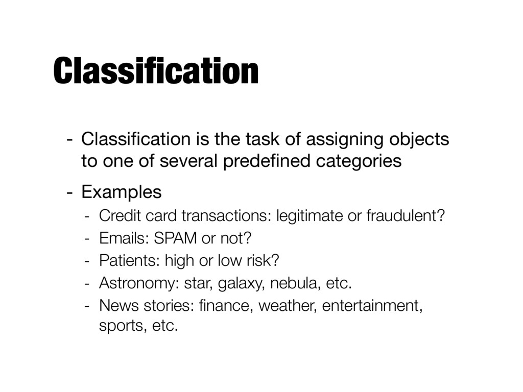
one of several predefined categories - Examples - Credit card transactions: legitimate or fraudulent? - Emails: SPAM or not? - Patients: high or low risk? - Astronomy: star, galaxy, nebula, etc. - News stories: finance, weather, entertainment, sports, etc.
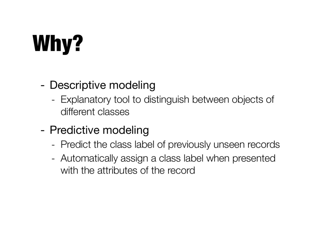
objects of different classes - Predictive modeling - Predict the class label of previously unseen records - Automatically assign a class label when presented with the attributes of the record
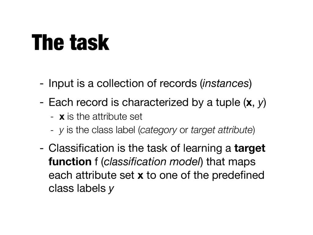
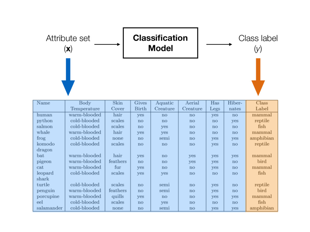
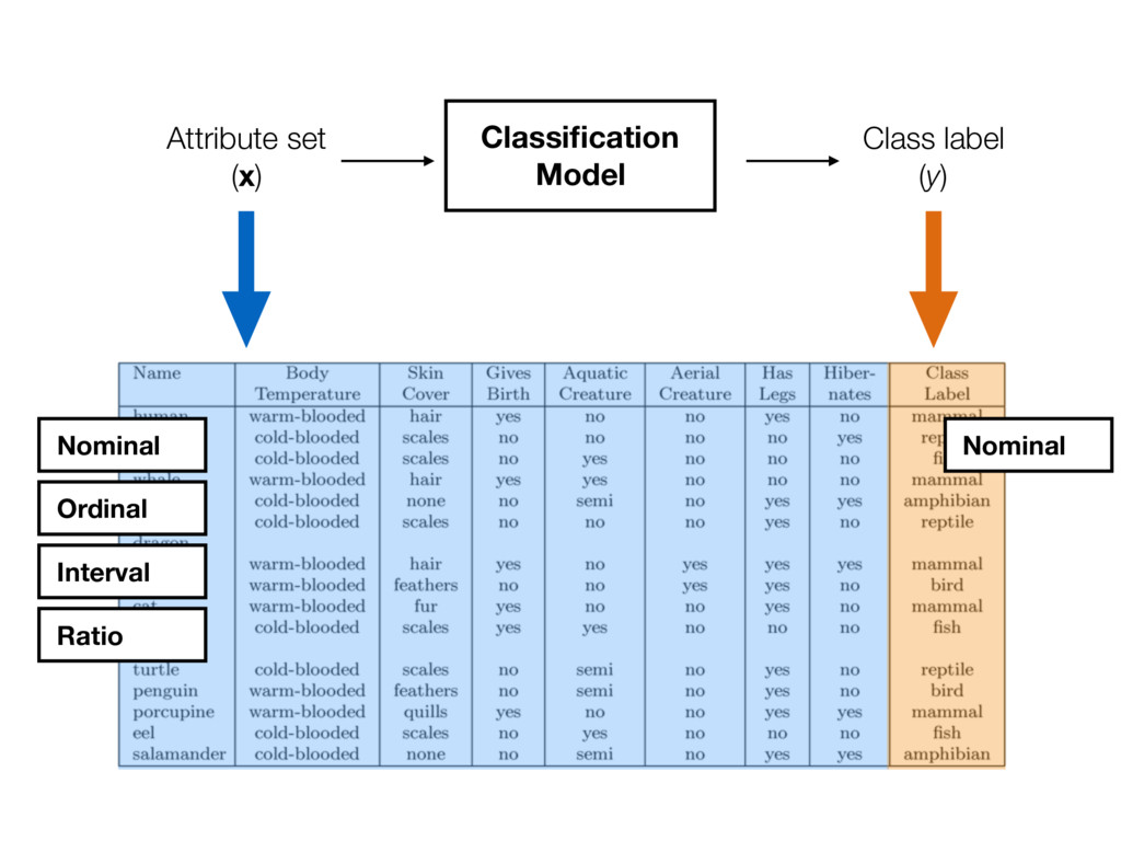
- Each record is characterized by a tuple (x, y) - x is the attribute set - y is the class label (category or target attribute) - Classification is the task of learning a target function f (classification model) that maps each attribute set x to one of the predefined class labels y
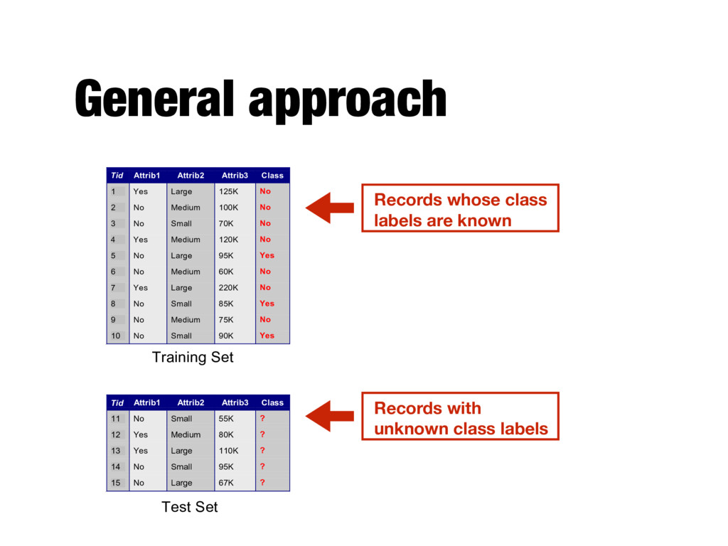
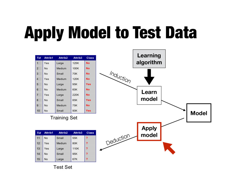
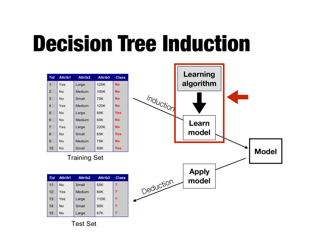
Attrib1 Attrib2 Attrib3 Class 1 Yes Large 125K No 2 No Medium 100K No 3 No Small 70K No 4 Yes Medium 120K No 5 No Large 95K Yes 6 No Medium 60K No 7 Yes Large 220K No 8 No Small 85K Yes 9 No Medium 75K No 10 No Small 90K Yes 10 Tid Attrib1 Attrib2 Attrib3 Class 11 No Small 55K ? 12 Yes Medium 80K ? 13 Yes Large 110K ? 14 No Small 95K ? 15 No Large 67K ? 10 Test Set Learning algorithm Training Set Records whose class labels are known Records with unknown class labels
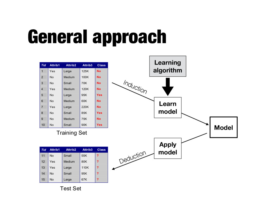
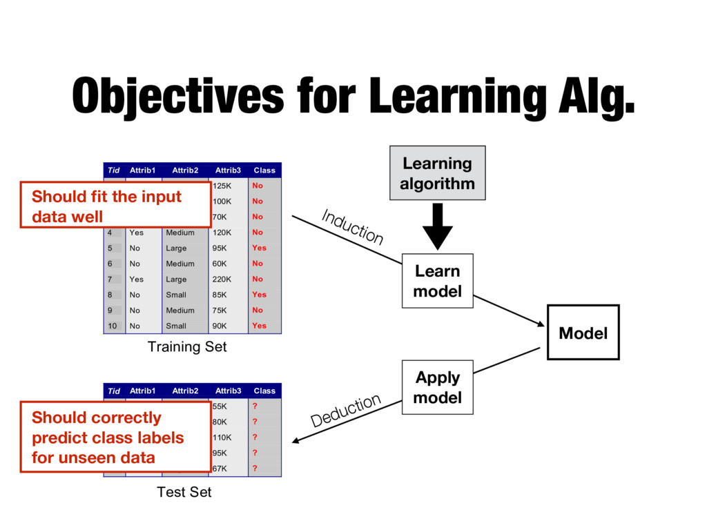
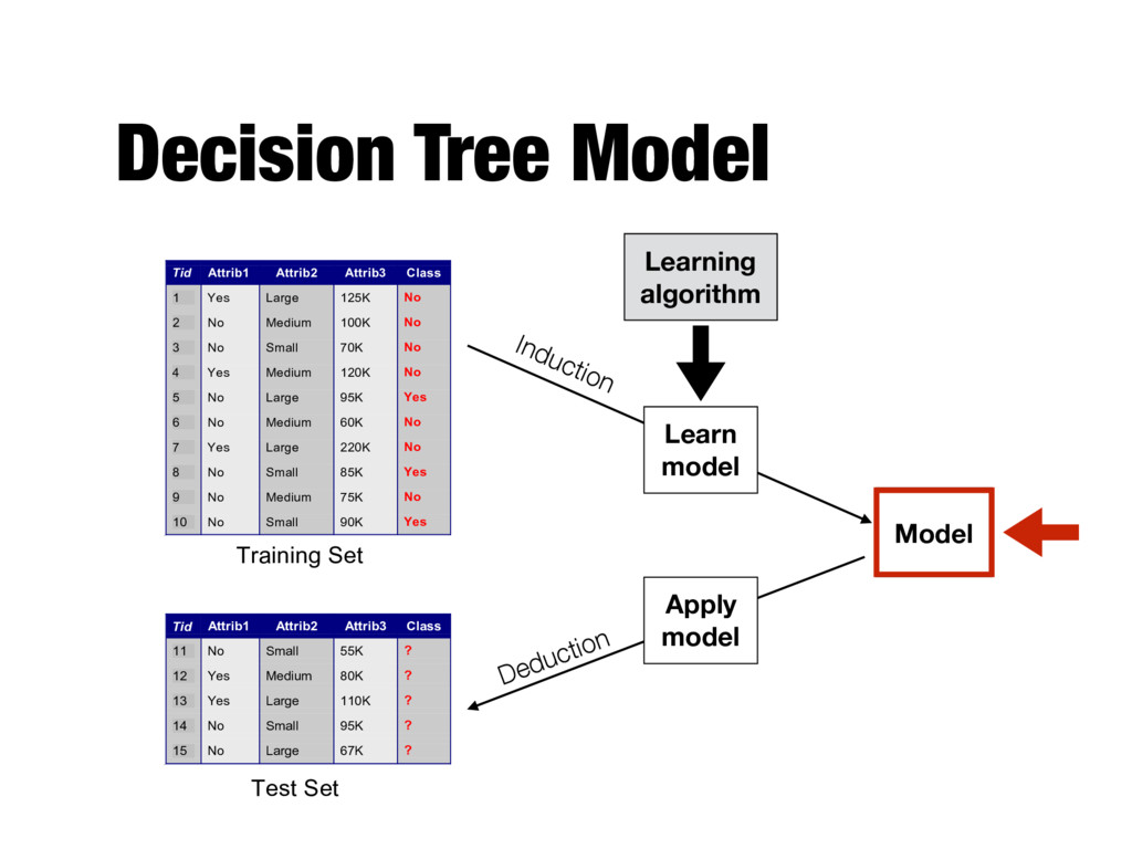
Attrib1 Attrib2 Attrib3 Class 1 Yes Large 125K No 2 No Medium 100K No 3 No Small 70K No 4 Yes Medium 120K No 5 No Large 95K Yes 6 No Medium 60K No 7 Yes Large 220K No 8 No Small 85K Yes 9 No Medium 75K No 10 No Small 90K Yes 10 Tid Attrib1 Attrib2 Attrib3 Class 11 No Small 55K ? 12 Yes Medium 80K ? 13 Yes Large 110K ? 14 No Small 95K ? 15 No Large 67K ? 10 Test Set Learning algorithm Training Set Model Learning algorithm Learn model Apply model Induction Deduction
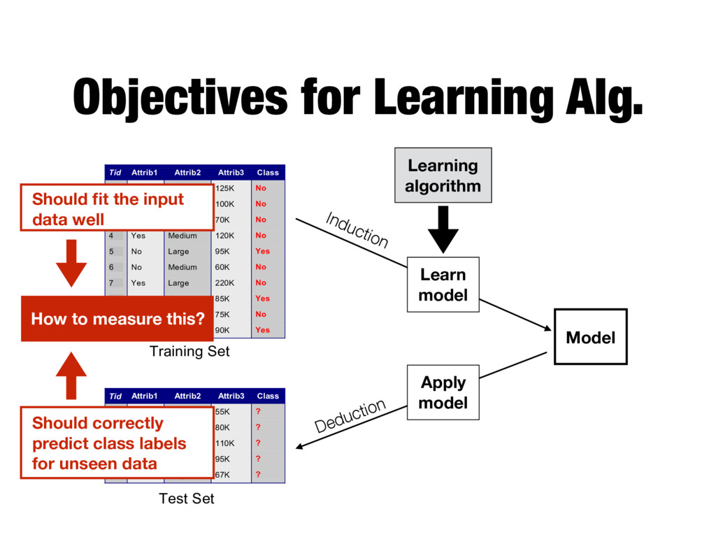
Model Tid Attrib1 Attrib2 Attrib3 Class 1 Yes Large 125K No 2 No Medium 100K No 3 No Small 70K No 4 Yes Medium 120K No 5 No Large 95K Yes 6 No Medium 60K No 7 Yes Large 220K No 8 No Small 85K Yes 9 No Medium 75K No 10 No Small 90K Yes 10 Tid Attrib1 Attrib2 Attrib3 Class 11 No Small 55K ? 12 Yes Medium 80K ? 13 Yes Large 110K ? 14 No Small 95K ? 15 No Large 67K ? 10 Test Set Learning algorithm Training Set Model Learning algorithm Learn model Apply model Induction Deduction Should fit the input data well Should correctly predict class labels for unseen data
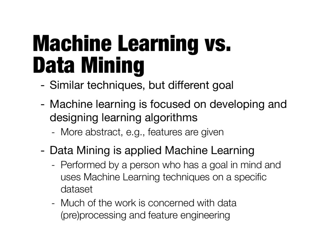
different goal - Machine learning is focused on developing and designing learning algorithms - More abstract, e.g., features are given - Data Mining is applied Machine Learning - Performed by a person who has a goal in mind and uses Machine Learning techniques on a specific dataset - Much of the work is concerned with data (pre)processing and feature engineering
Model Tid Attrib1 Attrib2 Attrib3 Class 1 Yes Large 125K No 2 No Medium 100K No 3 No Small 70K No 4 Yes Medium 120K No 5 No Large 95K Yes 6 No Medium 60K No 7 Yes Large 220K No 8 No Small 85K Yes 9 No Medium 75K No 10 No Small 90K Yes 10 Tid Attrib1 Attrib2 Attrib3 Class 11 No Small 55K ? 12 Yes Medium 80K ? 13 Yes Large 110K ? 14 No Small 95K ? 15 No Large 67K ? 10 Test Set Learning algorithm Training Set Model Learning algorithm Learn model Apply model Induction Deduction Should fit the input data well Should correctly predict class labels for unseen data How to measure this?
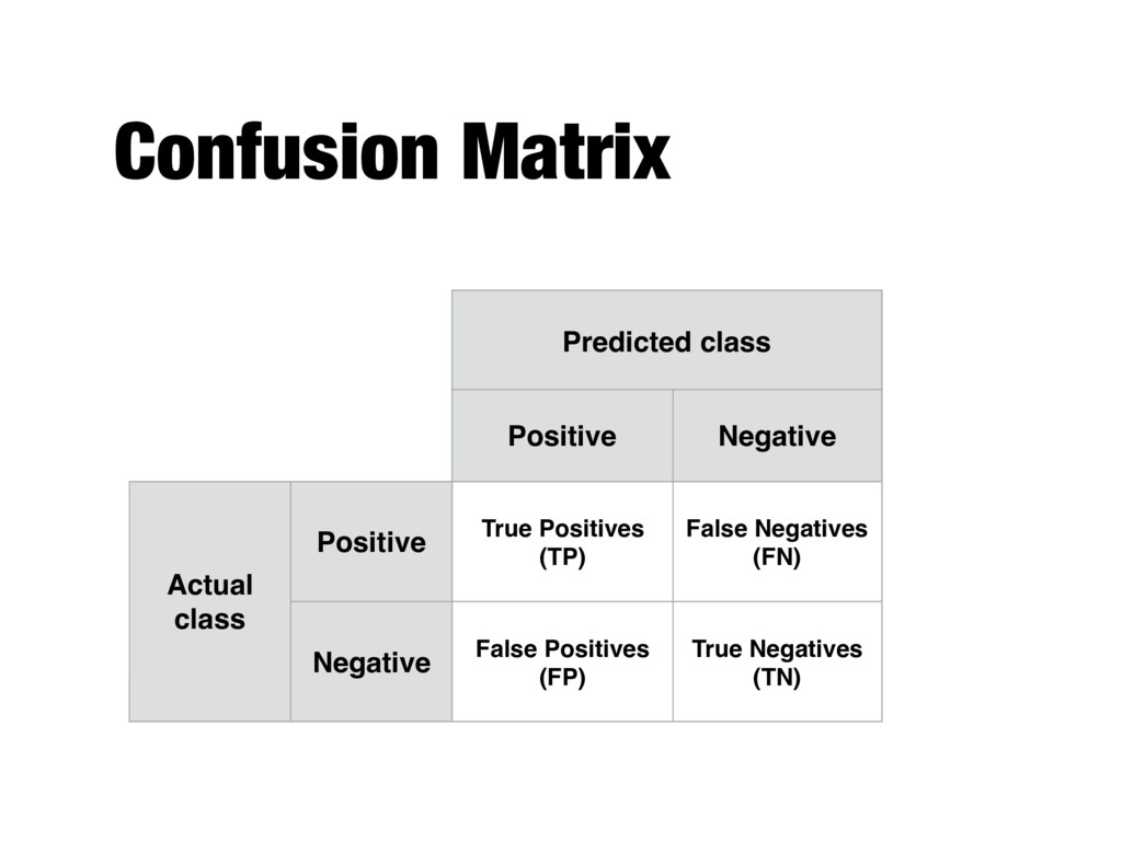
on the number of records correctly and incorrectly predicted by the model - Counts are tabulated in a table called the confusion matrix - Compute various performance metrics based on this matrix
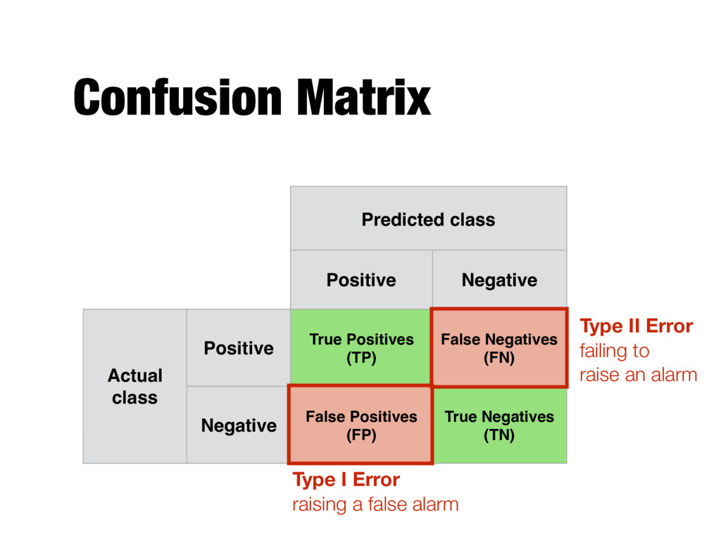
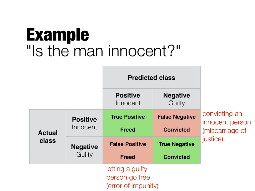
Positives (TP) False Negatives (FN) Negative False Positives (FP) True Negatives (TN) Type I Error raising a false alarm Type II Error failing to raise an alarm
Guilty Actual class Positive Innocent True Positive Freed False Negative Convicted Negative Guilty False Positive Freed True Negative Convicted convicting an innocent person (miscarriage of justice) letting a guilty person go free (error of impunity)
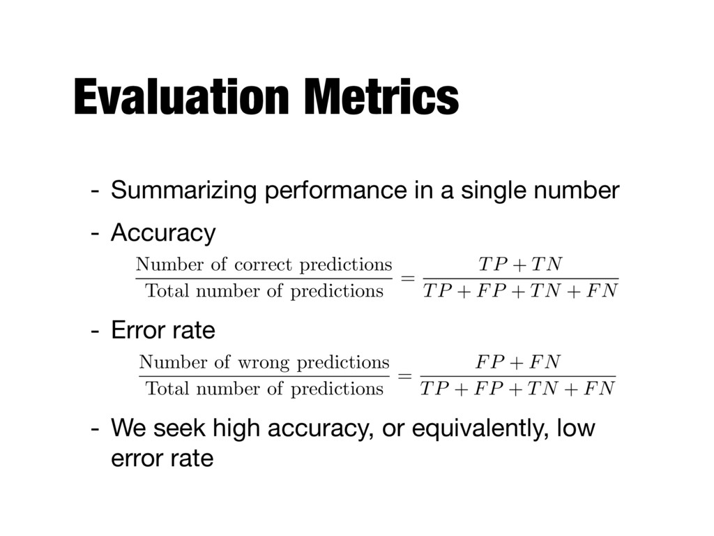
Accuracy - Error rate - We seek high accuracy, or equivalently, low error rate Number of correct predictions Total number of predictions = TP + TN TP + FP + TN + FN Number of wrong predictions Total number of predictions = FP + FN TP + FP + TN + FN
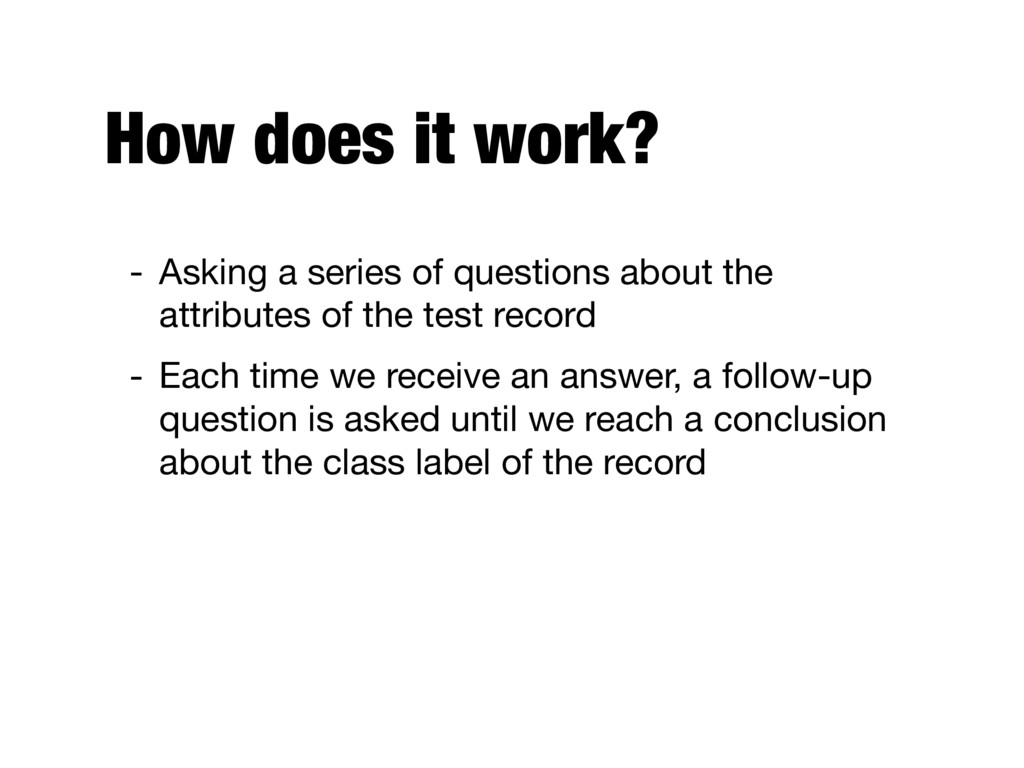
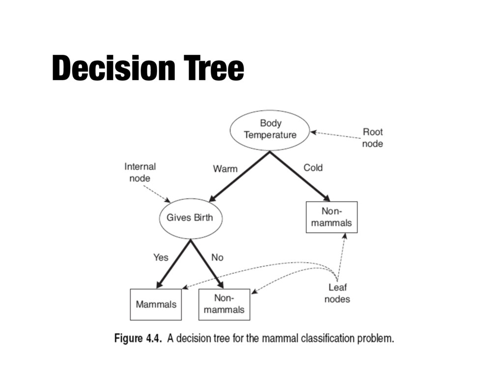
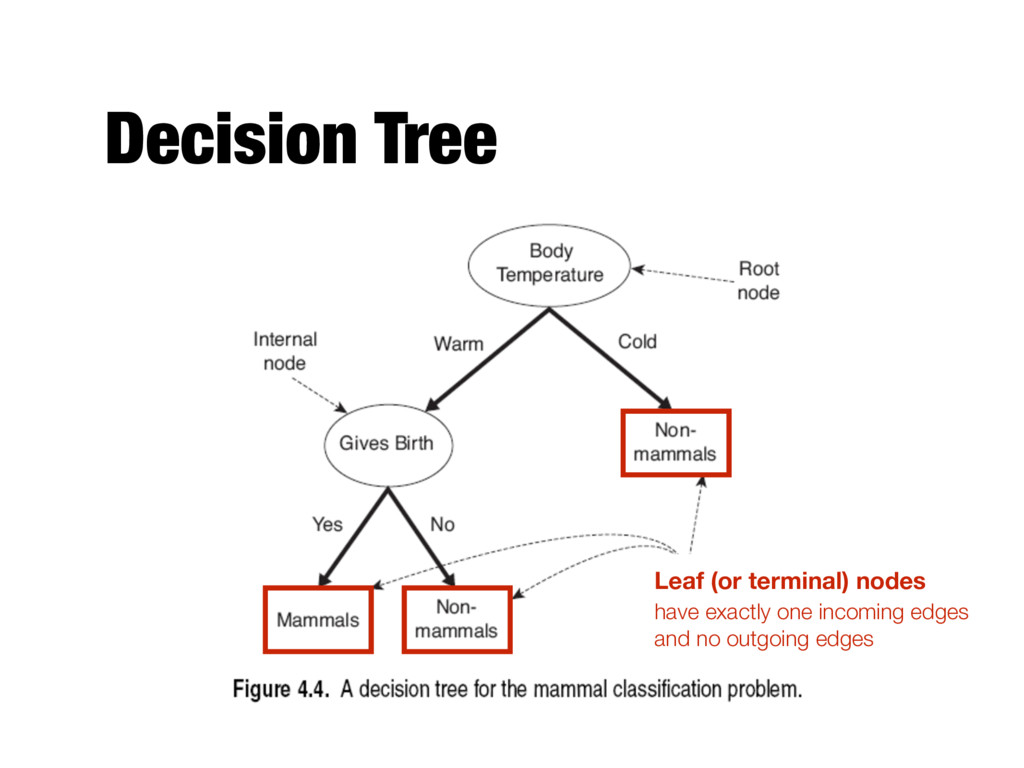
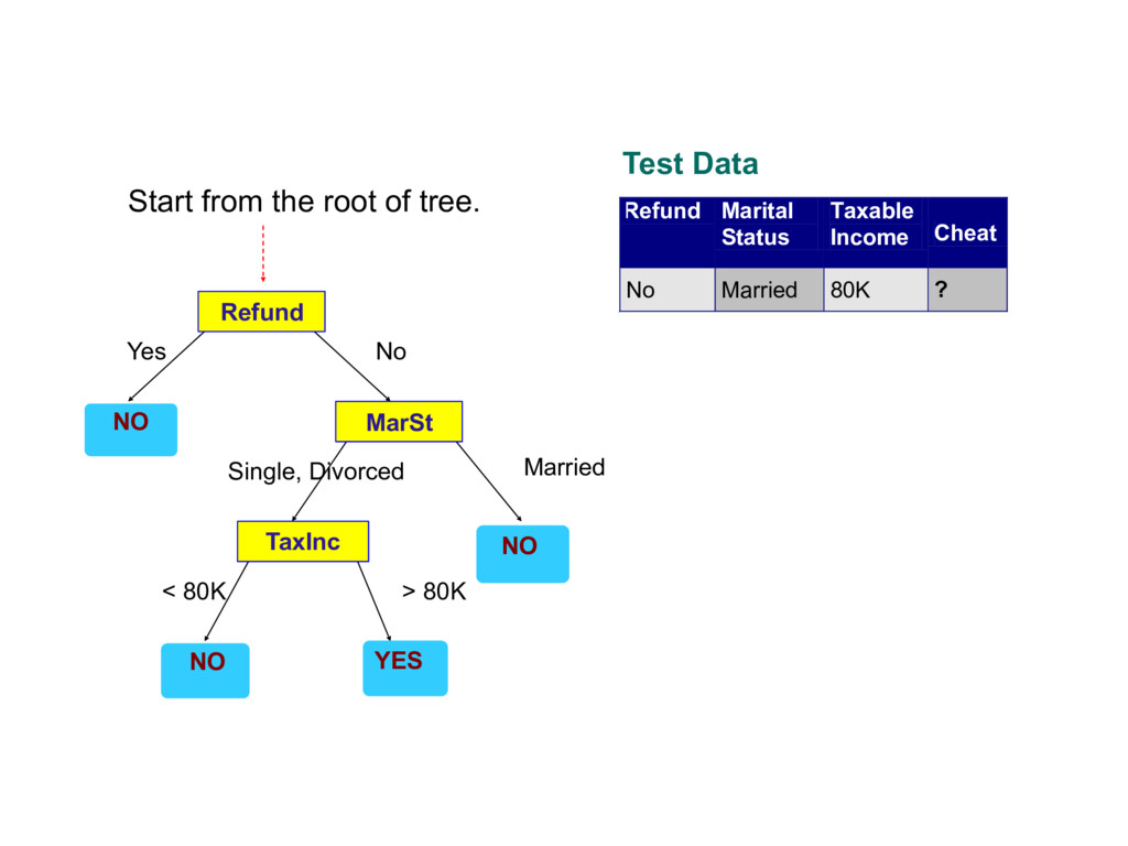
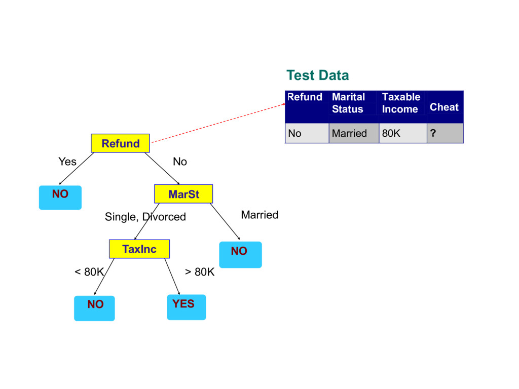
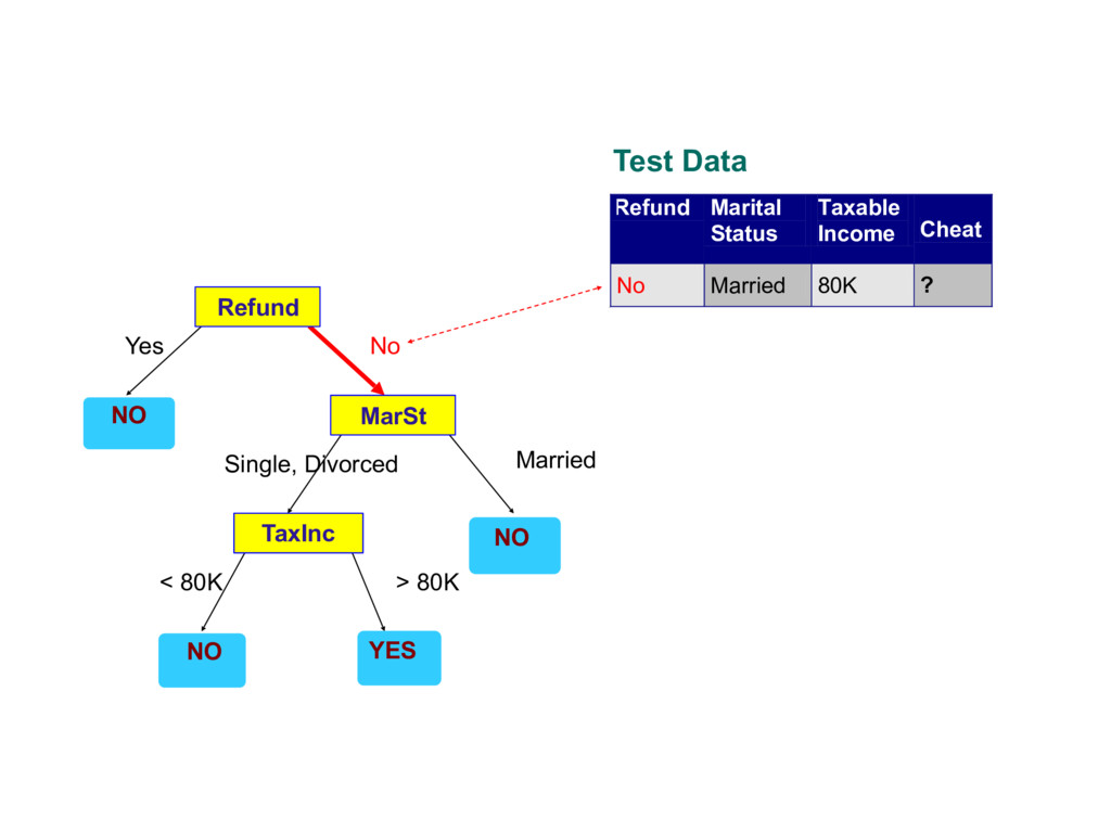
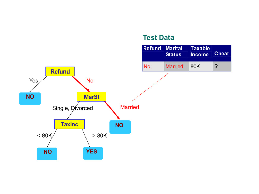
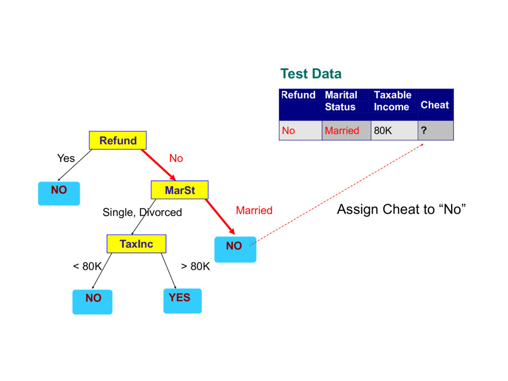
about the attributes of the test record - Each time we receive an answer, a follow-up question is asked until we reach a conclusion about the class label of the record
Tid Attrib1 Attrib2 Attrib3 Class 1 Yes Large 125K No 2 No Medium 100K No 3 No Small 70K No 4 Yes Medium 120K No 5 No Large 95K Yes 6 No Medium 60K No 7 Yes Large 220K No 8 No Small 85K Yes 9 No Medium 75K No 10 No Small 90K Yes 10 Tid Attrib1 Attrib2 Attrib3 Class 11 No Small 55K ? 12 Yes Medium 80K ? 13 Yes Large 110K ? 14 No Small 95K ? 15 No Large 67K ? 10 Test Set Learning algorithm Training Set Model Learning algorithm Learn model Apply model Induction Deduction
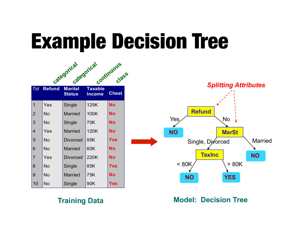
1 Yes Single 125K No 2 No Married 100K No 3 No Single 70K No 4 Yes Married 120K No 5 No Divorced 95K Yes 6 No Married 60K No 7 Yes Divorced 220K No 8 No Single 85K Yes 9 No Married 75K No 10 No Single 90K Yes 10 categorical categorical continuous class Refund MarSt TaxInc YES NO NO NO Yes No Married Single, Divorced < 80K > 80K Splitting Attributes Training Data Model: Decision Tree
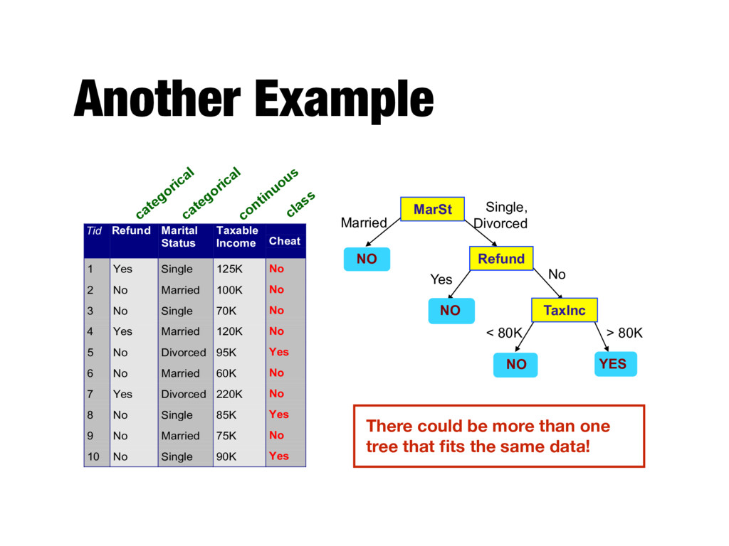
Yes Single 125K No 2 No Married 100K No 3 No Single 70K No 4 Yes Married 120K No 5 No Divorced 95K Yes 6 No Married 60K No 7 Yes Divorced 220K No 8 No Single 85K Yes 9 No Married 75K No 10 No Single 90K Yes 10 categorical categorical continuous class MarSt Refund TaxInc YES NO NO NO Yes No Married Single, Divorced < 80K > 80K There could be more than one tree that fits the same data!
Model Model Tid Attrib1 Attrib2 Attrib3 Class 1 Yes Large 125K No 2 No Medium 100K No 3 No Small 70K No 4 Yes Medium 120K No 5 No Large 95K Yes 6 No Medium 60K No 7 Yes Large 220K No 8 No Small 85K Yes 9 No Medium 75K No 10 No Small 90K Yes 10 Tid Attrib1 Attrib2 Attrib3 Class 11 No Small 55K ? 12 Yes Medium 80K ? 13 Yes Large 110K ? 14 No Small 95K ? 15 No Large 67K ? 10 Test Set Learning algorithm Training Set Model Learning algorithm Learn model Apply model Induction Deduction
Tid Attrib1 Attrib2 Attrib3 Class 1 Yes Large 125K No 2 No Medium 100K No 3 No Small 70K No 4 Yes Medium 120K No 5 No Large 95K Yes 6 No Medium 60K No 7 Yes Large 220K No 8 No Small 85K Yes 9 No Medium 75K No 10 No Small 90K Yes 10 Tid Attrib1 Attrib2 Attrib3 Class 11 No Small 55K ? 12 Yes Medium 80K ? 13 Yes Large 110K ? 14 No Small 95K ? 15 No Large 67K ? 10 Test Set Learning algorithm Training Set Model Learning algorithm Learn model Apply model Induction Deduction
can be constructed from a given set of attributes - Finding the optimal tree is computationally infeasible (NP-hard) - Greedy strategies are used - Grow a decision tree by making a series of locally optimum decisions about which attribute to use for splitting the data
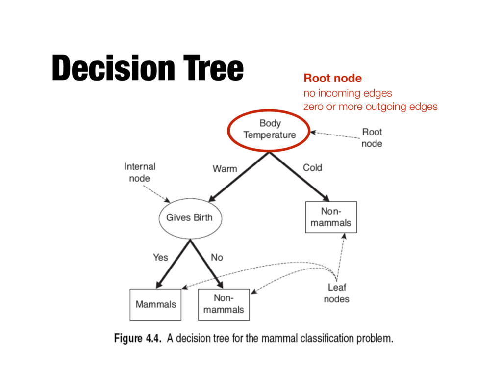
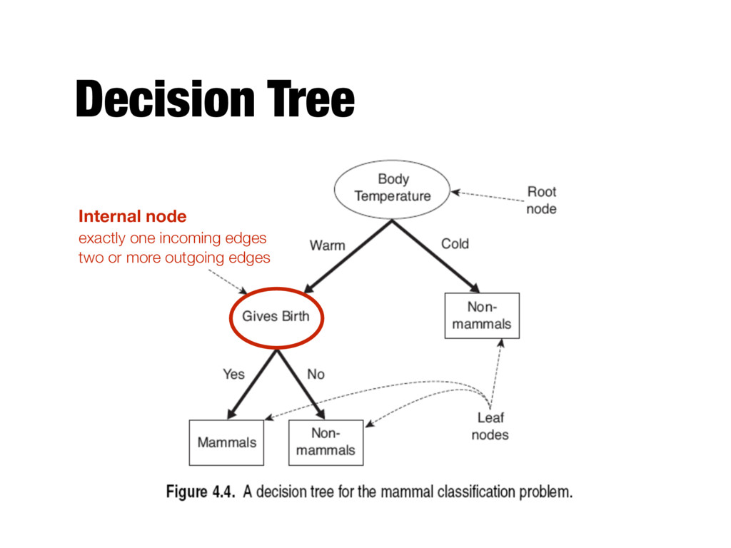
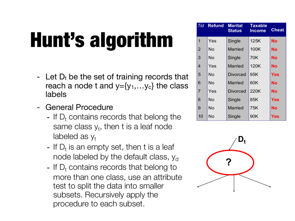
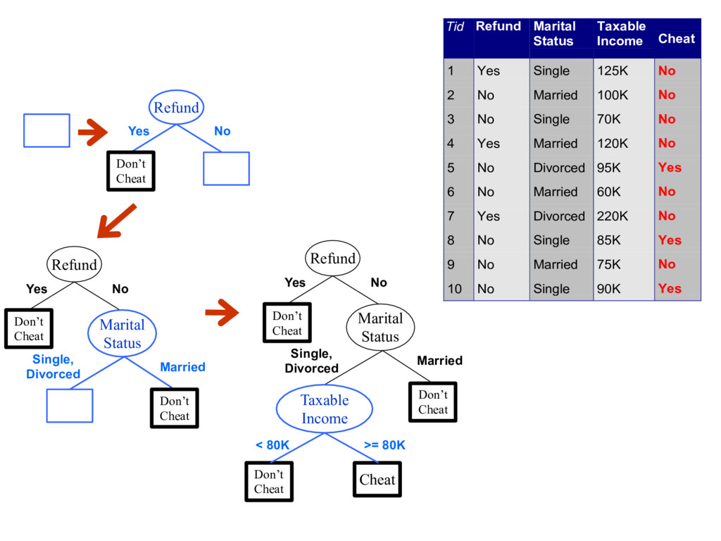
records that reach a node t and y={y1,…yc} the class labels - General Procedure - If Dt contains records that belong the same class yt , then t is a leaf node labeled as yt - If Dt is an empty set, then t is a leaf node labeled by the default class, yd - If Dt contains records that belong to more than one class, use an attribute test to split the data into smaller subsets. Recursively apply the procedure to each subset. Tid Refund Marital Status Taxable Income Cheat 1 Yes Single 125K No 2 No Married 100K No 3 No Single 70K No 4 Yes Married 120K No 5 No Divorced 95K Yes 6 No Married 60K No 7 Yes Divorced 220K No 8 No Single 85K Yes 9 No Married 75K No 10 No Single 90K Yes 10 Dt ?
Marital Status Don’t Cheat Cheat Single, Divorced Married Taxable Income Don’t Cheat < 80K >= 80K Refund Don’t Cheat Yes No Marital Status Don’t Cheat Single, Divorced Married Tid Refund Marital Status Taxable Income Cheat 1 Yes Single 125K No 2 No Married 100K No 3 No Single 70K No 4 Yes Married 120K No 5 No Divorced 95K Yes 6 No Married 60K No 7 Yes Divorced 220K No 8 No Single 85K Yes 9 No Married 75K No 10 No Single 90K Yes 10
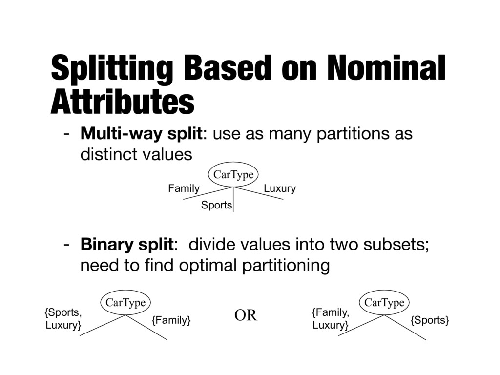
many partitions as distinct values - Binary split: divide values into two subsets; need to find optimal partitioning CarType Family Sports Luxury CarType {Family, Luxury} {Sports} CarType {Sports, Luxury} {Family} OR
many partitions as distinct values - Binary split: divides values into two subsets; need to find optimal partitioning Size Small Medium Large Size {Medium, Large} {Small} Size {Small, Medium} {Large} OR
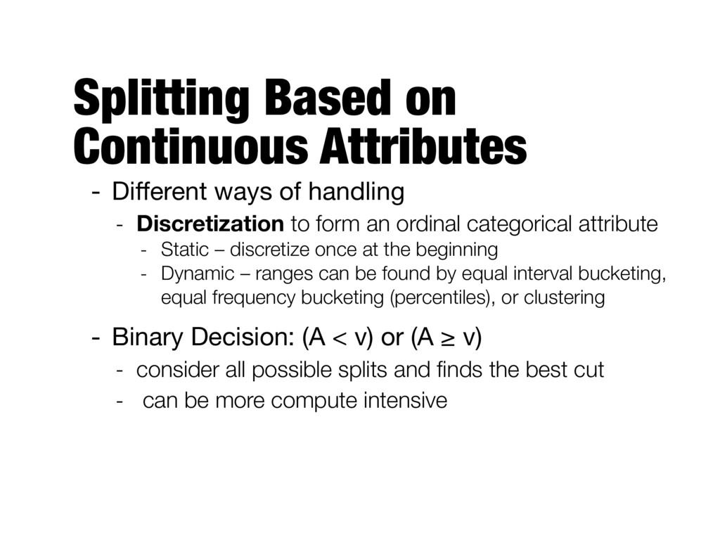
- Discretization to form an ordinal categorical attribute - Static – discretize once at the beginning - Dynamic – ranges can be found by equal interval bucketing, equal frequency bucketing (percentiles), or clustering - Binary Decision: (A < v) or (A ≥ v) - consider all possible splits and finds the best cut - can be more compute intensive
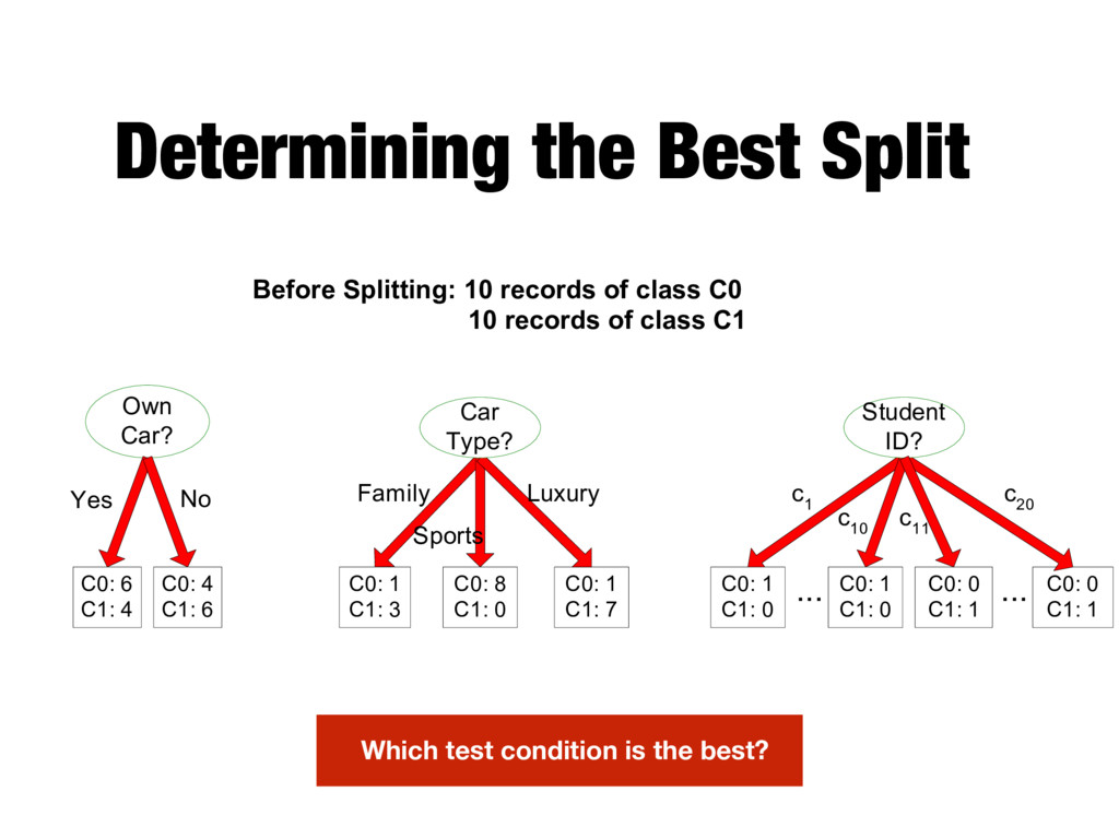
C0: 4 C1: 6 C0: 1 C1: 3 C0: 8 C1: 0 C0: 1 C1: 7 Car Type? C0: 1 C1: 0 C0: 1 C1: 0 C0: 0 C1: 1 Student ID? ... Yes No Family Sports Luxury c 1 c 10 c 20 C0: 0 C1: 1 ... c 11 Before Splitting: 10 records of class C0 10 records of class C1 Which test condition is the best?
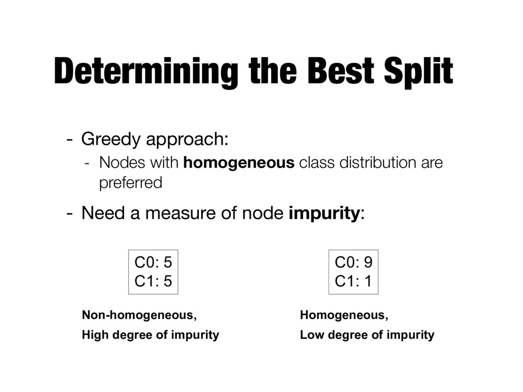
homogeneous class distribution are preferred - Need a measure of node impurity: C0: 5 C1: 5 C0: 9 C1: 1 Non-homogeneous, High degree of impurity Homogeneous, Low degree of impurity
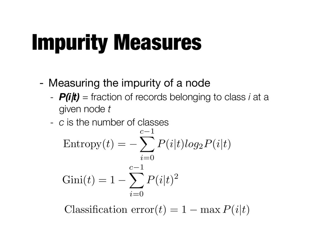
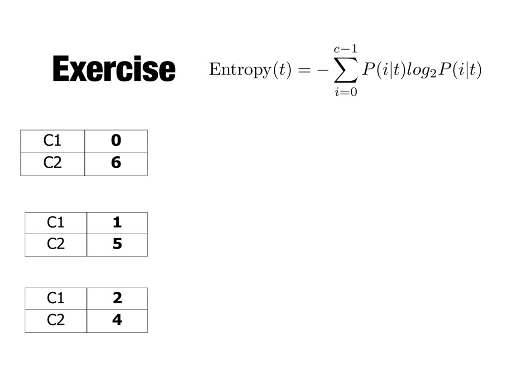
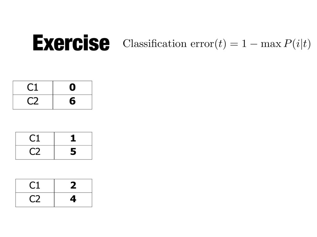
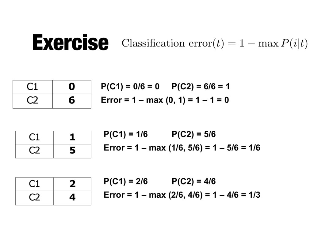
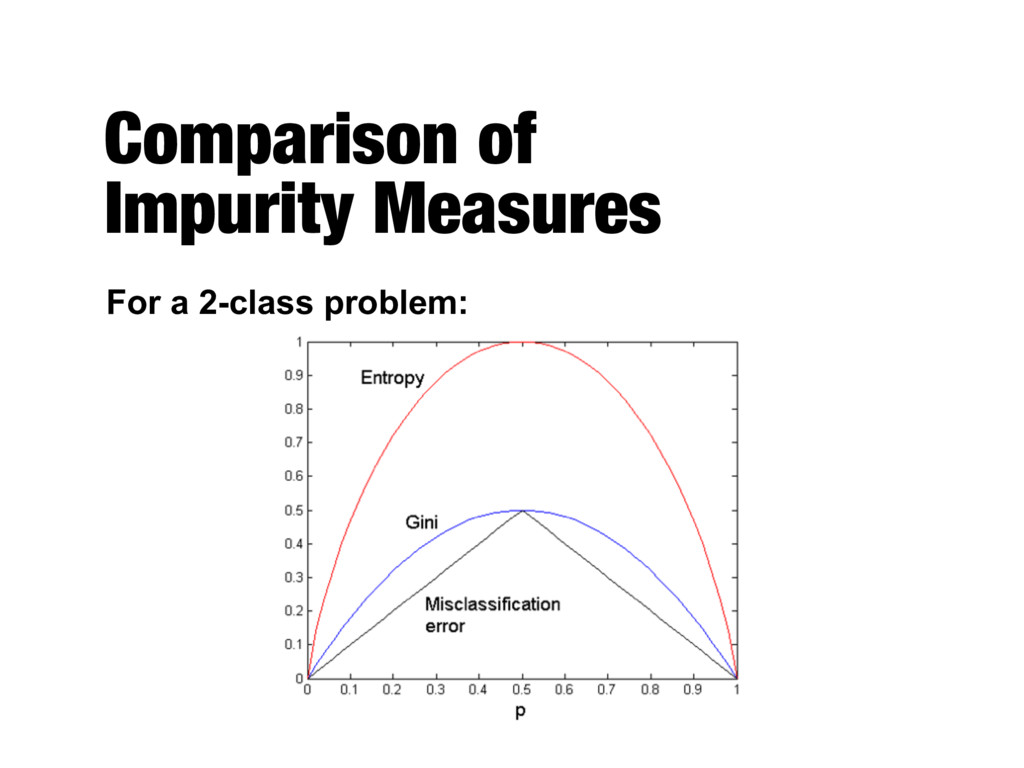
P(i|t) = fraction of records belonging to class i at a given node t - c is the number of classes Entropy(t) = c 1 X i=0 P(i | t)log2P(i | t) Classification error( t ) = 1 max P ( i|t ) Gini(t) = 1 c 1 X i=0 P(i|t)2
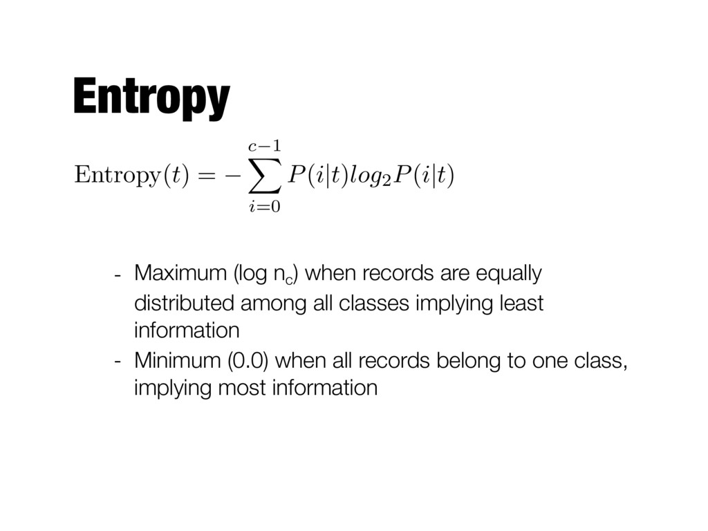
| t) - Maximum (log nc ) when records are equally distributed among all classes implying least information - Minimum (0.0) when all records belong to one class, implying most information
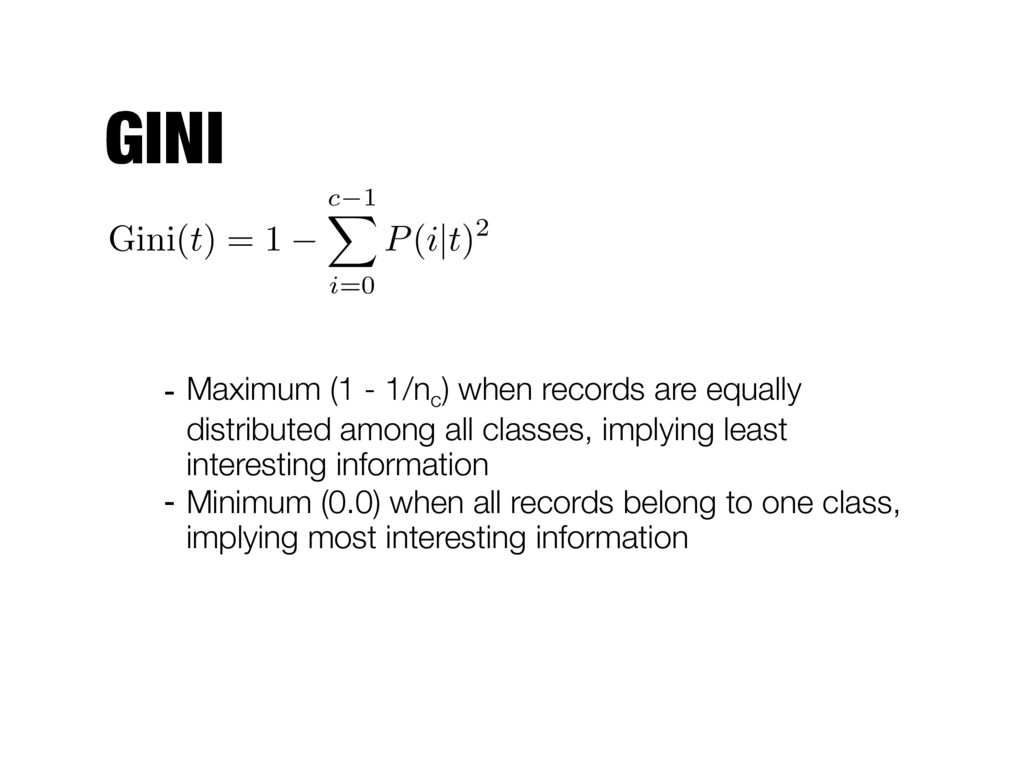
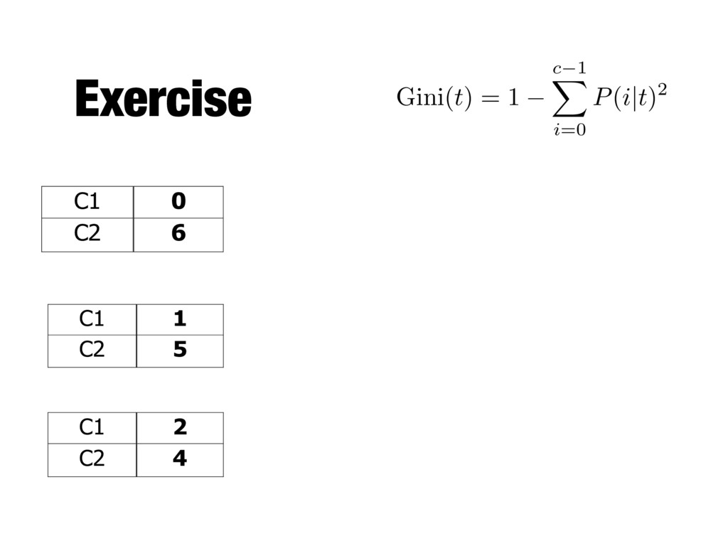
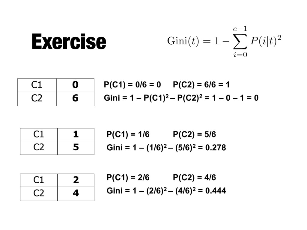
equally distributed among all classes, implying least interesting information - Minimum (0.0) when all records belong to one class, implying most interesting information Gini(t) = 1 c 1 X i=0 P(i|t)2
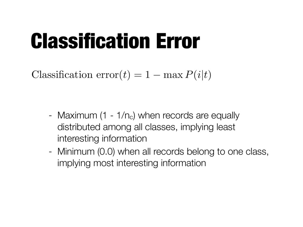
( i|t ) - Maximum (1 - 1/nc) when records are equally distributed among all classes, implying least interesting information - Minimum (0.0) when all records belong to one class, implying most interesting information
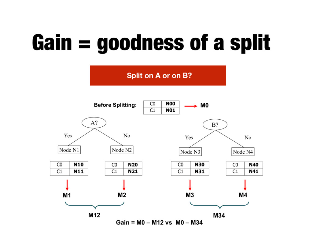
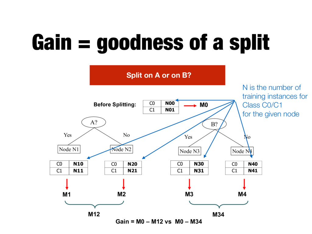
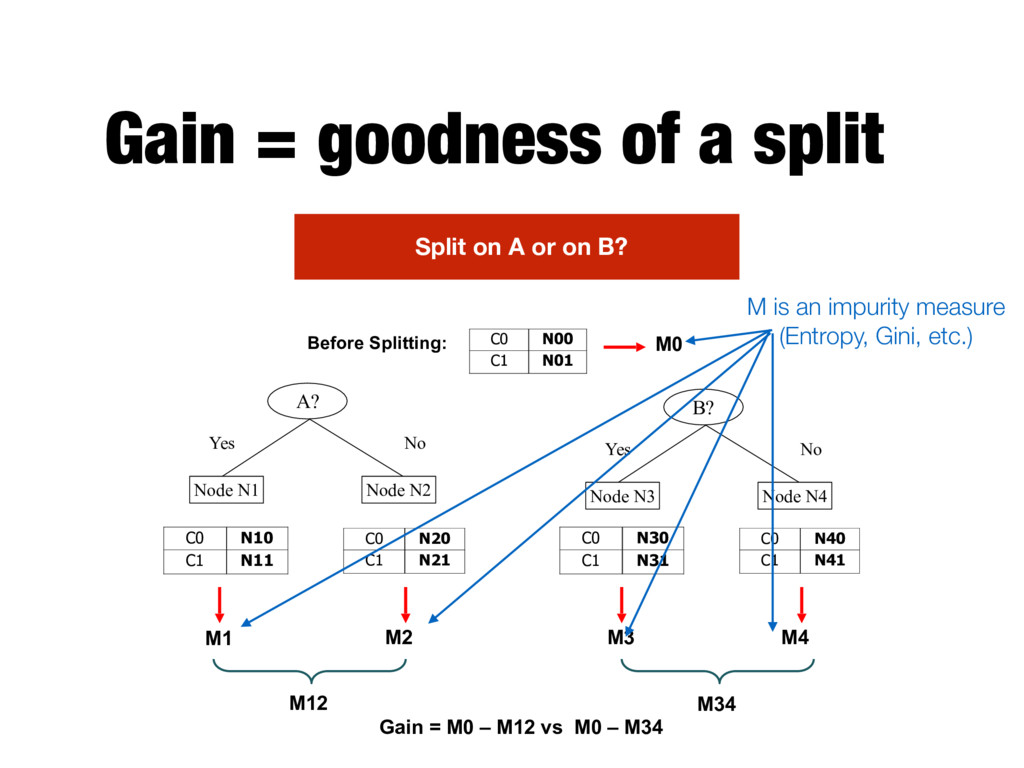
N3 Node N4 A? Yes No Node N1 Node N2 Before Splitting: C0 N10 C1 N11 C0 N20 C1 N21 C0 N30 C1 N31 C0 N40 C1 N41 C0 N00 C1 N01 M0 M1 M2 M3 M4 M12 M34 Gain = M0 – M12 vs M0 – M34 Split on A or on B? N is the number of training instances for Class C0/C1 for the given node
N3 Node N4 A? Yes No Node N1 Node N2 Before Splitting: C0 N10 C1 N11 C0 N20 C1 N21 C0 N30 C1 N31 C0 N40 C1 N41 C0 N00 C1 N01 M0 M1 M2 M3 M4 M12 M34 Gain = M0 – M12 vs M0 – M34 Split on A or on B? The node that produces the higher gain is considered the better split
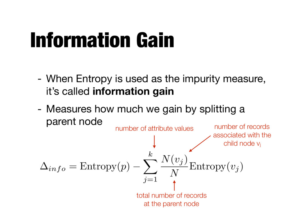
measure, it’s called information gain - Measures how much we gain by splitting a parent node number of attribute values total number of records at the parent node number of records associated with the child node vj info = Entropy( p ) k X j =1 N ( v j) N Entropy( v j)
C0: 4 C1: 6 C0: 1 C1: 3 C0: 8 C1: 0 C0: 1 C1: 7 Car Type? C0: 1 C1: 0 C0: 1 C1: 0 C0: 0 C1: 1 Student ID? ... Yes No Family Sports Luxury c 1 c 10 c 20 C0: 0 C1: 1 ... c 11 Before Splitting: 10 records of class C0 10 records of class C1 Which test condition is the best?
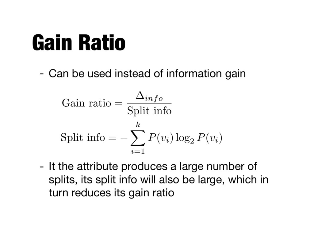
of splits, its split info will also be large, which in turn reduces its gain ratio Gain ratio = info Split info Split info = k X i=1 P ( vi) log2 P ( vi) - Can be used instead of information gain
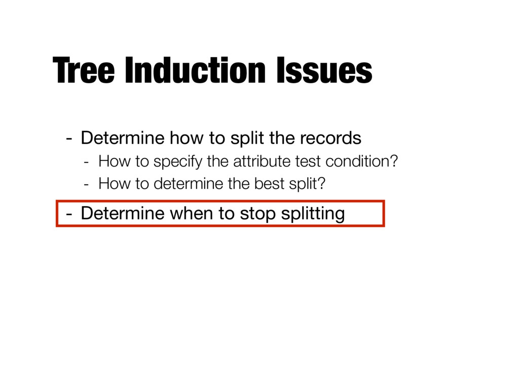
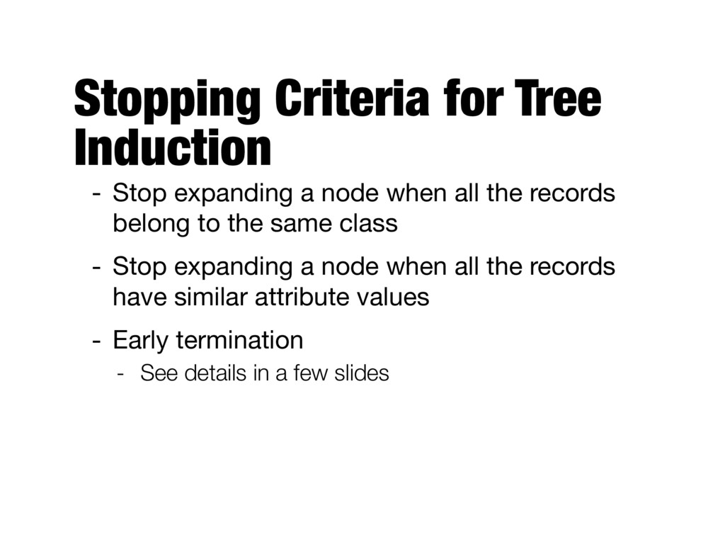
when all the records belong to the same class - Stop expanding a node when all the records have similar attribute values - Early termination - See details in a few slides
at classifying unknown records - Easy to interpret for small-sized trees - Accuracy is comparable to other classification techniques for many simple data sets
Model Tid Attrib1 Attrib2 Attrib3 Class 1 Yes Large 125K No 2 No Medium 100K No 3 No Small 70K No 4 Yes Medium 120K No 5 No Large 95K Yes 6 No Medium 60K No 7 Yes Large 220K No 8 No Small 85K Yes 9 No Medium 75K No 10 No Small 90K Yes 10 Tid Attrib1 Attrib2 Attrib3 Class 11 No Small 55K ? 12 Yes Medium 80K ? 13 Yes Large 110K ? 14 No Small 95K ? 15 No Large 67K ? 10 Test Set Learning algorithm Training Set Model Learning algorithm Learn model Apply model Induction Deduction Should fit the input data well Should correctly predict class labels for unseen data
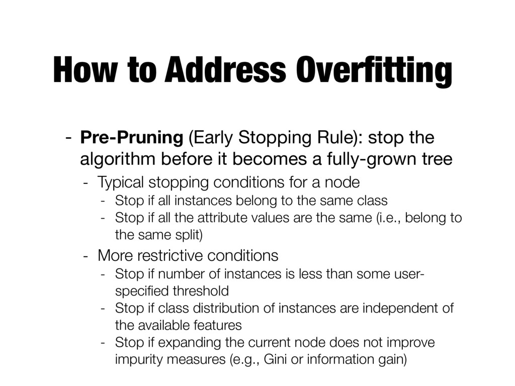
the algorithm before it becomes a fully-grown tree - Typical stopping conditions for a node - Stop if all instances belong to the same class - Stop if all the attribute values are the same (i.e., belong to the same split) - More restrictive conditions - Stop if number of instances is less than some user- specified threshold - Stop if class distribution of instances are independent of the available features - Stop if expanding the current node does not improve impurity measures (e.g., Gini or information gain)
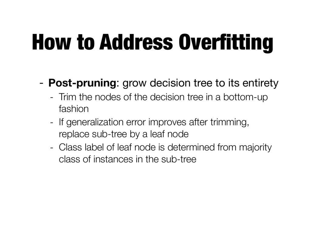
its entirety - Trim the nodes of the decision tree in a bottom-up fashion - If generalization error improves after trimming, replace sub-tree by a leaf node - Class label of leaf node is determined from majority class of instances in the sub-tree
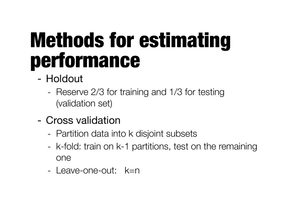
training and 1/3 for testing (validation set) - Cross validation - Partition data into k disjoint subsets - k-fold: train on k-1 partitions, test on the remaining one - Leave-one-out: k=n