Information Retrieval and Text Mining - Information Retrieval (Part III)

University of Stavanger, DAT640, 2019 fall

Transcript

1. Informa on Retrieval (Part III) [DAT640] Informa on Retrieval and Text Mining Krisz an Balog University of Stavanger September 23, 2019
2. Outline • Search engine architecture, indexing • Evaluation • Retrieval models ⇐ today • Query modeling • Learning-to-rank, Neural IR • Semantic search 2 / 37
3. So far • Document retrieval task: scoring documents against a search query • Inverted index: special data structure to facilitate large-scale retrieval • Evaluation: measuring the goodness of a ranking against the ground truth using binary or graded relevance 3 / 37
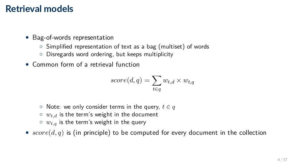
4. Retrieval models • Bag-of-words representation ◦ Simplified representation of text as a bag (multiset) of words ◦ Disregards word ordering, but keeps multiplicity • Common form of a retrieval function score(d, q) = t∈q wt,d × wt,q ◦ Note: we only consider terms in the query, t ∈ q ◦ wt,d is the term’s weight in the document ◦ wt,q is the term’s weight in the query • score(d, q) is (in principle) to be computed for every document in the collection 4 / 37
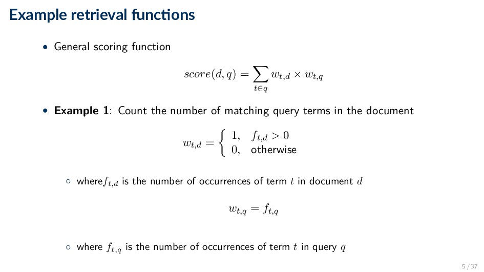
5. Example retrieval func ons • General scoring function score(d, q) = t∈q wt,d × wt,q • Example 1: Count the number of matching query terms in the document wt,d = 1, ft,d > 0 0, otherwise ◦ whereft,d is the number of occurrences of term t in document d wt,q = ft,q ◦ where ft,q is the number of occurrences of term t in query q 5 / 37
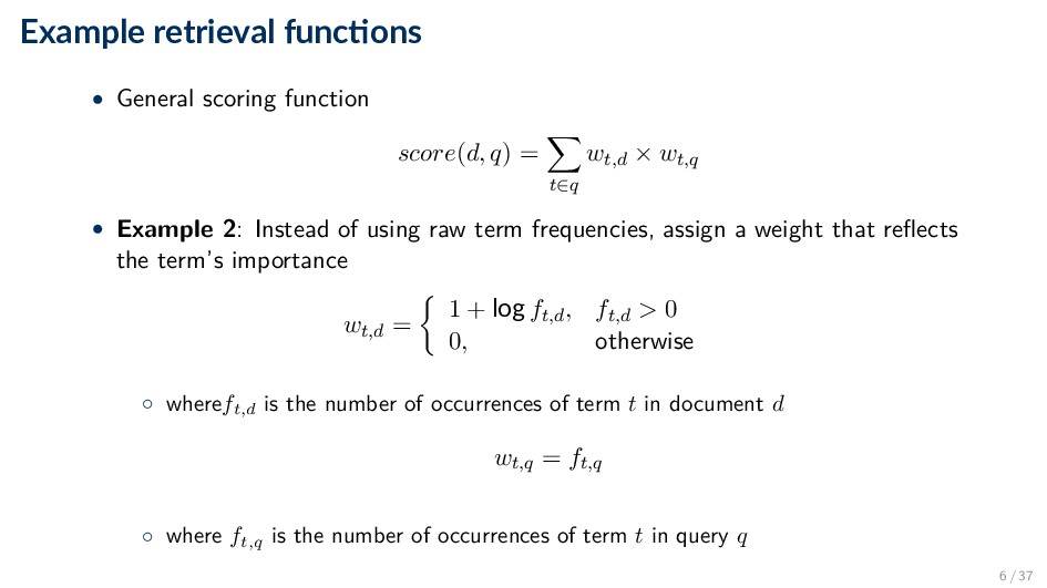
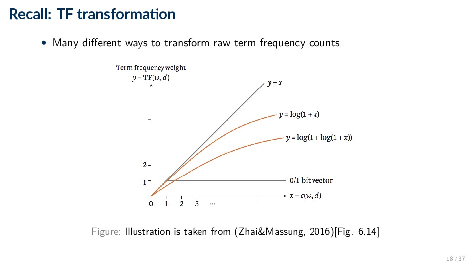
6. Example retrieval func ons • General scoring function score(d, q) = t∈q wt,d × wt,q • Example 2: Instead of using raw term frequencies, assign a weight that reflects the term’s importance wt,d = 1 + log ft,d, ft,d > 0 0, otherwise ◦ whereft,d is the number of occurrences of term t in document d wt,q = ft,q ◦ where ft,q is the number of occurrences of term t in query q 6 / 37
7. Vector Space Model 7 / 37
8. Vector space model • Basis of most IR research in the 1960s and 70s • Still used • Provides a simple and intuitively appealing framework for implementing ◦ Term weighting ◦ Ranking ◦ Relevance feedback 8 / 37
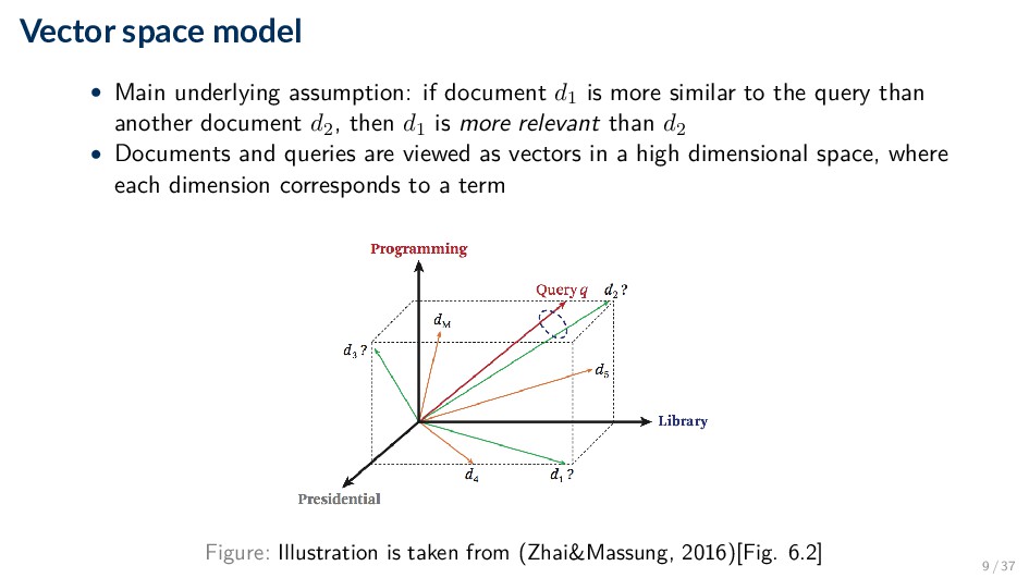
9. Vector space model • Main underlying assumption: if document d1 is more similar to the query than another document d2, then d1 is more relevant than d2 • Documents and queries are viewed as vectors in a high dimensional space, where each dimension corresponds to a term Figure: Illustration is taken from (Zhai&Massung, 2016)[Fig. 6.2] 9 / 37
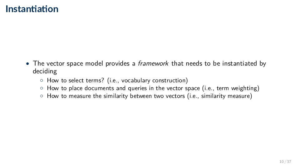
10. Instan a on • The vector space model provides a framework that needs to be instantiated by deciding ◦ How to select terms? (i.e., vocabulary construction) ◦ How to place documents and queries in the vector space (i.e., term weighting) ◦ How to measure the similarity between two vectors (i.e., similarity measure) 10 / 37
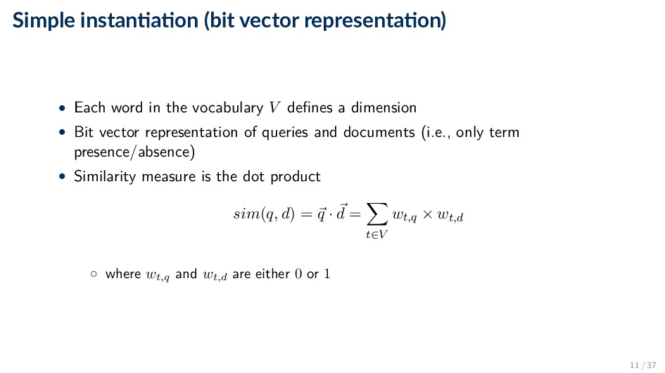
11. Simple instan a on (bit vector representa on) • Each word in the vocabulary V defines a dimension • Bit vector representation of queries and documents (i.e., only term presence/absence) • Similarity measure is the dot product sim(q, d) = q · d = t∈V wt,q × wt,d ◦ where wt,q and wt,d are either 0 or 1 11 / 37
12. Discussion Question What are potential shortcomings of this simple instantiation? 12 / 37
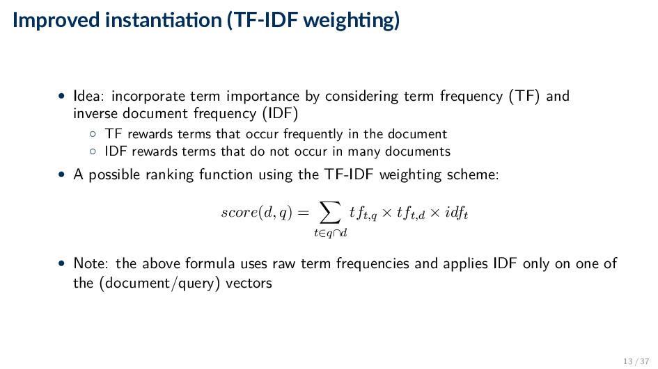
13. Improved instan a on (TF-IDF weigh ng) • Idea: incorporate term importance by considering term frequency (TF) and inverse document frequency (IDF) ◦ TF rewards terms that occur frequently in the document ◦ IDF rewards terms that do not occur in many documents • A possible ranking function using the TF-IDF weighting scheme: score(d, q) = t∈q∩d tft,q × tft,d × idft • Note: the above formula uses raw term frequencies and applies IDF only on one of the (document/query) vectors 13 / 37
14. Many different variants out there! • Different variants of TF and IDF • Different TF-IDF weighting for the query and for the document • Different similarity measure (e.g., cosine) 14 / 37
15. Exercise #1 • Implement vector space retrieval • Code skeleton on GitHub: exercises/lecture_09/exercise_1.ipynb (make a local copy) 15 / 37
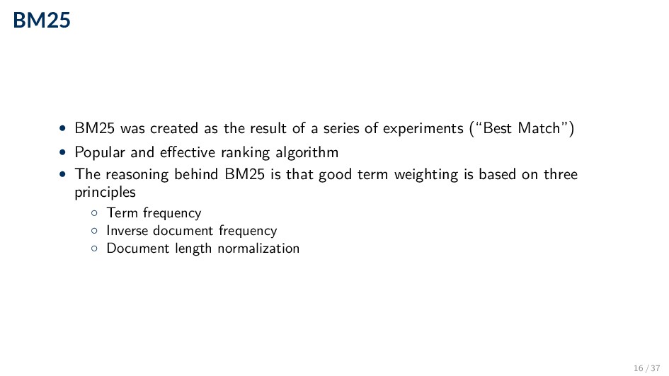
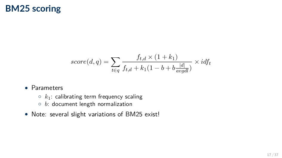
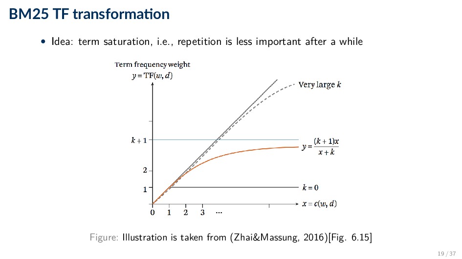
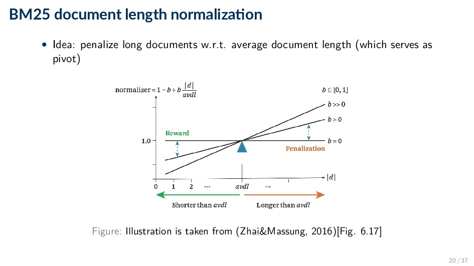
16. BM25 • BM25 was created as the result of a series of experiments (“Best Match”) • Popular and effective ranking algorithm • The reasoning behind BM25 is that good term weighting is based on three principles ◦ Term frequency ◦ Inverse document frequency ◦ Document length normalization 16 / 37
17. BM25 scoring score(d, q) = t∈q ft,d × (1 + k1) ft,d + k1(1 − b + b |d| avgdl ) × idft • Parameters ◦ k1 : calibrating term frequency scaling ◦ b: document length normalization • Note: several slight variations of BM25 exist! 17 / 37
18. Recall: TF transforma on • Many different ways to transform raw term frequency counts Figure: Illustration is taken from (Zhai&Massung, 2016)[Fig. 6.14] 18 / 37
19. BM25 TF transforma on • Idea: term saturation, i.e., repetition is less important after a while Figure: Illustration is taken from (Zhai&Massung, 2016)[Fig. 6.15] 19 / 37
20. BM25 document length normaliza on • Idea: penalize long documents w.r.t. average document length (which serves as pivot) Figure: Illustration is taken from (Zhai&Massung, 2016)[Fig. 6.17] 20 / 37
21. BM25 parameter se ng • k1: calibrating term frequency scaling ◦ 0 corresponds to a binary model ◦ large values correspond to using raw term frequencies ◦ typical values are between 1.2 and 2.0; a common default value is 1.2 • b: document length normalization ◦ 0: no normalization at all ◦ 1: full length normalization ◦ typical value: 0.75 21 / 37
22. Language Models 22 / 37
23. Language models • Based on the notion of probabilities and processes for generating text • Wide range of usage across different applications ◦ Speech recognition • “I ate a cherry” is a more likely sentence than “Eye eight uh Jerry” ◦ OCR and handwriting recognition • More probable sentences are more likely correct readings ◦ Machine translation • More likely sentences are probably better translations 23 / 37
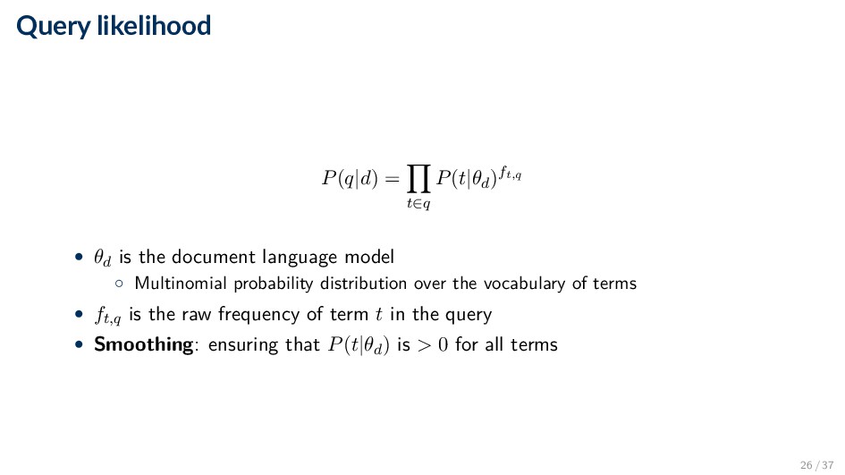
24. Language models for ranking documents • Represent each document as a multinomial probability distribution over terms • Estimate the probability that the query was “generated” by the given document ◦ How likely is the search query given the language model of the document? 24 / 37
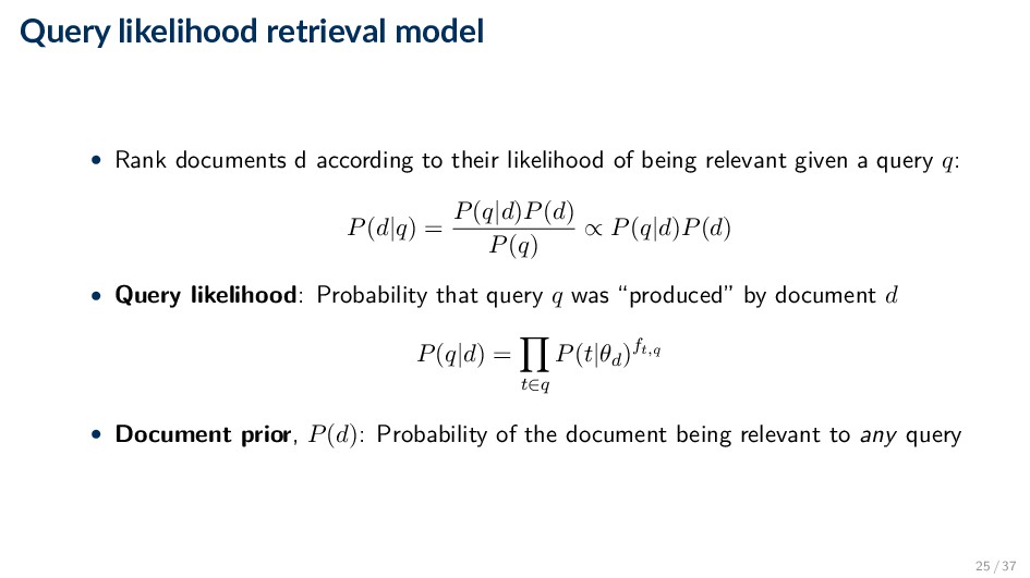
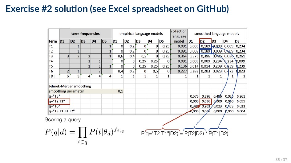
25. Query likelihood retrieval model • Rank documents d according to their likelihood of being relevant given a query q: P(d|q) = P(q|d)P(d) P(q) ∝ P(q|d)P(d) • Query likelihood: Probability that query q was “produced” by document d P(q|d) = t∈q P(t|θd)ft,q • Document prior, P(d): Probability of the document being relevant to any query 25 / 37
26. Query likelihood P(q|d) = t∈q P(t|θd)ft,q • θd is the document language model ◦ Multinomial probability distribution over the vocabulary of terms • ft,q is the raw frequency of term t in the query • Smoothing: ensuring that P(t|θd) is > 0 for all terms 26 / 37
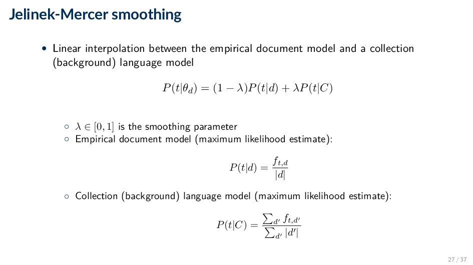
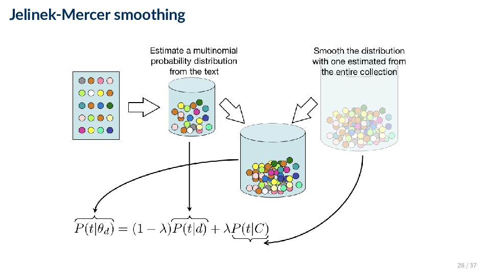
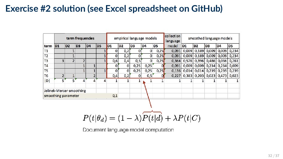
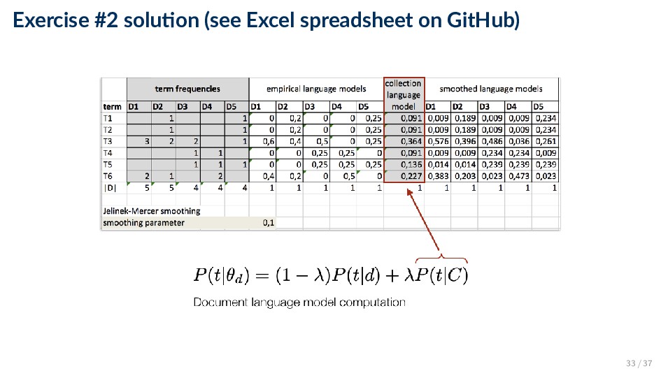
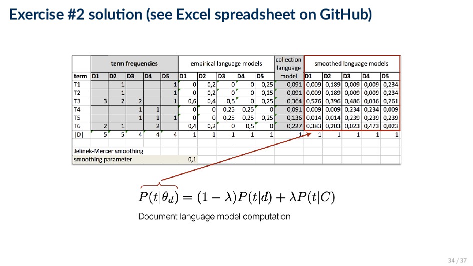
27. Jelinek-Mercer smoothing • Linear interpolation between the empirical document model and a collection (background) language model P(t|θd) = (1 − λ)P(t|d) + λP(t|C) ◦ λ ∈ [0, 1] is the smoothing parameter ◦ Empirical document model (maximum likelihood estimate): P(t|d) = ft,d |d| ◦ Collection (background) language model (maximum likelihood estimate): P(t|C) = d ft,d d |d | 27 / 37
28. Jelinek-Mercer smoothing 28 / 37
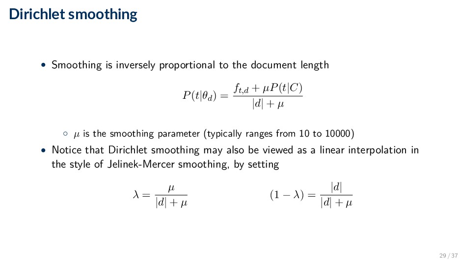
29. Dirichlet smoothing • Smoothing is inversely proportional to the document length P(t|θd) = ft,d + µP(t|C) |d| + µ ◦ µ is the smoothing parameter (typically ranges from 10 to 10000) • Notice that Dirichlet smoothing may also be viewed as a linear interpolation in the style of Jelinek-Mercer smoothing, by setting λ = µ |d| + µ (1 − λ) = |d| |d| + µ 29 / 37
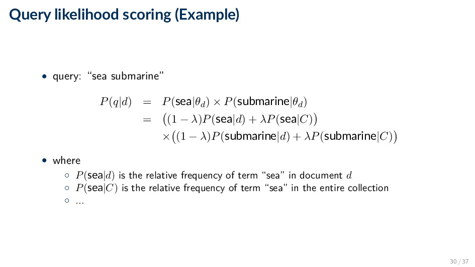
30. Query likelihood scoring (Example) • query: “sea submarine” P(q|d) = P(sea|θd) × P(submarine|θd) = (1 − λ)P(sea|d) + λP(sea|C) × (1 − λ)P(submarine|d) + λP(submarine|C) • where ◦ P(sea|d) is the relative frequency of term “sea” in document d ◦ P(sea|C) is the relative frequency of term “sea” in the entire collection ◦ ... 30 / 37
31. Exercise #2 • Document retrieval using language models (paper-based) 31 / 37
32. Exercise #2 solu on (see Excel spreadsheet on GitHub) 32 / 37
33. Exercise #2 solu on (see Excel spreadsheet on GitHub) 33 / 37
34. Exercise #2 solu on (see Excel spreadsheet on GitHub) 34 / 37
35. Exercise #2 solu on (see Excel spreadsheet on GitHub) 35 / 37
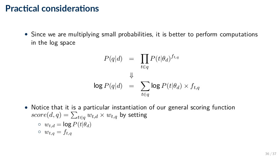
36. Prac cal considera ons • Since we are multiplying small probabilities, it is better to perform computations in the log space P(q|d) = t∈q P(t|θd)ft,q ⇓ log P(q|d) = t∈q log P(t|θd) × ft,q • Notice that it is a particular instantiation of our general scoring function score(d, q) = t∈q wt,d × wt,q by setting ◦ wt,d = log P(t|θd ) ◦ wt,q = ft,q 36 / 37
37. Reading • Text Data Management and Analysis (Zhai&Massung), Chapter 6 37 / 37