Practical Query Tuning in PostgreSQL

Slow queries can be a common challenge when working with PostgreSQL, and understanding how to identify and resolve performance bottlenecks is key to maintaining a high-performing database.
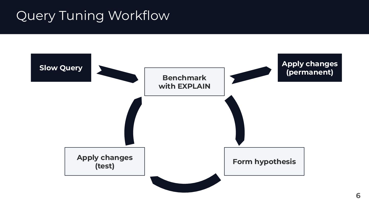
In this talk, we'll dive into practical examples that demonstrate how to diagnose performance bottlenecks using tools like EXPLAIN and optimize queries effectively. Using relatable and actionable scenarios, we'll walk through common causes of slow queries, how to analyze execution plans, and practical steps for improvement, such as optimizing indexes and rewriting queries. We'll also explore the impact of statistics and planner decisions—key factors in understanding why PostgreSQL chooses a particular execution plan.
This session is designed for those who are familiar with the basics of reading EXPLAIN plans and want to expand their skills by applying them to practical scenarios.

Transcript

1. Practical Query Tuning in PostgreSQL From Diagnosis to Optimization PGDay Chicago 2025 April 25, 2025 Keiko Oda - pganalyze
2. Table of Contents • Query Tuning Workflow ◦ How to find a slow query? ◦ Benchmarking with EXPLAIN • EXPLAIN Refresher ◦ Recap basics • Case 1: Missing Index ◦ Statistics, Selectivity and Index • Case 2: ORDER BY with LIMIT ◦ My query got slow without touching it! • Case 3: Nested Loop with misestimate ◦ JOIN types and order 2
3. Speaker Intro • Keiko Oda • Product Engineer at pganalyze ◦ Sponsoring! Say hi at our booth! • From Japan ◦ Kanazawa, Ishikawa ◦ The 25 best places in the world to travel to in 2025 by National Geographic 3 I love beers! Let me know if you have any recommendations in Chicago
4. Speaker Intro • Keiko Oda • Product Engineer at pganalyze ◦ Sponsoring! Say hi at our booth! • From Japan ◦ Kanazawa, Ishikawa ◦ The 25 best places in the world to travel to in 2025 by National Geographic 4 I love beers! Let me know if you have any recommendations in Chicago Map source: JAIST https://www.jaist.ac.jp/english/top/access/
5. Query Tuning Workflow 5
6. Query Tuning Workflow 6 Form hypothesis Apply changes (test) Slow Query Apply changes (permanent) Benchmark with EXPLAIN
7. Query Tuning Workflow 7 Form hypothesis Apply changes (test) Slow Query Apply changes (permanent) Benchmark with EXPLAIN
8. How to find a slow query? • Application performance monitoring (APM) tools ◦ Which endpoint or job is slow? ◦ Using trace views to pinpoint slow parts of the request 8
9. How to find a slow query? • Isolate issues ◦ System level: “Is the query slow, or is the system overloaded”? ◦ Database level (locks, etc.): “Is the query slow, or it is waiting for something else”? 9
10. How to find a slow query? • Isolate issues ◦ System level: “Is the query slow, or is the system overloaded”? ◦ Database level (locks, etc.): “Is the query slow, or it is waiting for something else”? 10
11. How to find a slow query? • pg_stat_statements ◦ Tracks query execution stats (total time, call counts, rows, I/O metrics) 11
12. Postgres Platform "Best Practices" for the Modern DBA 📹-3 How to find more info of a slow query? • log_min_duration_statement (config) ◦ Logs all queries that run longer than the specified duration (e.g. 1000ms) • auto_explain (extension) ◦ Automatically logs the EXPLAIN output of slow queries ▪ It’s supported by most cloud providers and relatively easy to set up ◦ auto_explain configuration options ▪ auto_explain supports many of the same options as the EXPLAIN commands ▪ auto_explain.log_min_duration ▪ auto_explain.log_analyze: Runs EXPLAIN ANALYZE - ON recommended ▪ auto_explain.log_buffers: Runs EXPLAIN BUFFERS - ON recommended ▪ auto_explain.log_timing: OFF as a starter, ON if possible ◦ “Prioritize observability > latency” - by Chelsea Dole 12 Collect Postgres EXPLAIN plans using auto_explain 📖-4
13. Query Tuning Workflow 13 Form hypothesis Apply changes (test) Slow Query Apply changes (permanent) Benchmark with EXPLAIN
14. Benchmarking with EXPLAIN • Use EXPLAIN ANALYZE to measure the baseline ◦ If possible, enable BUFFERS (ON by default with ANALYZE from 18), VERBOSE, I/O Timing (track_io_timing) for more detailed insights • Run EXPLAIN multiple times to reduce cold cache effects ◦ The first run can be affected by cache, making it unstable as a benchmark ▪ Cold cache: Disk I/O, buffer cache, CPU overhead, etc. ◦ Important part: measure the benchmark under the same condition ◦ Use pg_buffercache_evict_all() function (new from 18) • Benchmark with different parameter sets ◦ The same query may use different plans depending on the parameter values ◦ A query improvement for one parameter set might hurt performance for others 14
15. pg_buffercache_evict and pg_buffercache_evict_all • pg_buffercache_evict() ◦ New in Postgres 17 ◦ Need to specify the buffer ID • pg_buffercache_evict_all() ◦ New in Postgres 18 ◦ Evict all cache in shared buffers ◦ Do not run this in production 15 Understanding Postgres IOPS: Why They Matter Even When Everything Fits in Cache 📖-2 Hit Read
16. EXPLAIN Refresher Recap basics 16
17. What is EXPLAIN? EXPLAIN will show a plan tree the Planner picked 17 Parser Rewriter Planner Executor SELECT id, name FROM users WHERE org_id = 123; id | name ----+------- 1 | Alice 3 | Beth 7 | Emily Plan tree Query tree Query Result Tweaked Query tree Plan tree 1 Plan tree 2 Plan tree 3
18. Planner’s role Planner’s role: Creating an optimal execution plan 1. Consider all(-ish) possible plans for a given query ◦ Whether to use an index or not, which join types to use, and in what order to join tables ◦ In some cases, it doesn’t explore all possible plans (will take too long for planning) 2. Calculate the cost of each plan ◦ Cost: internal unit of effort to compare different execution plans ◦ e.g. Sequential pages are more expensive (seq_page_cost) than cached/indexed pages (random_page_cost) 3. Choose the plan with the lowest estimated cost 18
19. When the query is slow… The planner is not picking up “the best” plan • Bad estimates: Stats are stale or too basic • Missing options: No index = no chance to use one • Cost can be tricky: What looks cheap might not be cheap (or fast) • Query shape matters: CTEs, functions, etc. can block optimization 19 Planner Plan tree 1 Plan tree 2 Plan tree 3
20. Cheapest cost != fastest 20
21. Case 1: Missing Index Statistics, Selectivity and Index 21
22. Statistics • Postgres maintains statistics per table ◦ Statistics are per-column by default ▪ multi-column statistics (extended stats) can be created with CREATE STATISTICS ◦ Collected automatically by autovacuum(analyze) or manually with ANALYZE 22 A Deep Dive into Postgres Statistics 📹-5 column avg_width Average width of the column’s values n_distinct Estimated number of distinct values (-1 indicates all values are unique) most_common_vals A list of the most common values in the column histogram_bounds A list of values that divide the column’s values into approx. equally sized groups
23. Statistics 23 SELECT attname, avg_width, n_distinct, most_common_vals, histogram_bounds FROM pg_stats WHERE tablename = 'postgres_roles' AND attname IN ('create_db', 'connection_limit'); -[ RECORD 1 ]----+----------------------------------------------------------------------------- attname | connection_limit avg_width | 4 n_distinct | 27 most_common_vals | {-1,20,5,10} histogram_bounds | {0,0,1,3,3,6,6,30,30,40,50,50,75,100,100,200,325,500,500,999,1000,1024,2000} -[ RECORD 2 ]----+----------------------------------------------------------------------------- attname | create_db avg_width | 1 n_distinct | 2 most_common_vals | {f,t} histogram_bounds | The pg_stats system view
24. Selectivity and Index • Selectivity: How many rows match a given search condition ◦ High selectivity (few rows match) → Planner may choose Index Scan ◦ Low selectivity (many rows match) → Planner may prefer Sequential Scan • Not all indexes are worth creating ◦ Low selectivity may be ignored + write overhead and storage cost 24 Postgres' Clever Query Planning System 📖-3
25. Test data ☕ 25 CREATE TABLE products( id int not null, name text not null, PRIMARY KEY(id) ); INSERT INTO products (id, name) VALUES (1, 'Latte'), (2, 'Espresso'), (3, 'Cappuccino'), (4, 'Americano'), (5, 'Mocha'); ANALYZE products; ☕ Table: products
26. Test data 🧾 26 CREATE TABLE orders( id int not null, product_id int not null, user_id int not null, created_at date not null, PRIMARY KEY (id) ); INSERT INTO orders (id, product_id, user_id, created_at) SELECT generate_series(1, 5000000) AS id, -- 5M orders floor(random() * 5 + 1)::int AS product_id, -- No “users” table, but assuming there are 100k users by issuing 1-100k user IDs floor(random() * 100000 + 1)::int AS user_id, -- 100k users (about ~50 orders per user) date '2024-01-01' + (random() * 365)::int AS created_at; ANALYZE orders; 🧾 Table: orders
27. Missing index 27 EXPLAIN ANALYZE SELECT count(*) FROM orders WHERE product_id = 5; QUERY PLAN ------------------------------------------------------------------------------------------------------------------- Finalize Aggregate (cost=55117.28..55117.29 rows=1 width=8) (actual time=106.312..106.978 rows=1 loops=1) -> Gather (cost=55117.06..55117.27 rows=2 width=8) (actual time=106.271..106.972 rows=3 loops=1) Workers Planned: 2 Workers Launched: 2 -> Partial Aggregate (cost=54117.06..54117.07 rows=1 width=8) (actual time=99.692..99.692 rows=1 loops=3) -> Parallel Seq Scan on orders (cost=0.00..53069.67 rows=418958 width=0) (actual time=0.138..88.288 rows=333854 loops=3) Filter: (product_id = 5) Rows Removed by Filter: 1332813 Planning Time: 0.487 ms Execution Time: 107.031 ms (10 rows) Total order count of Mocha (product_id = 5)
28. Missing index 28 EXPLAIN ANALYZE SELECT count(*) FROM orders WHERE product_id = 5; QUERY PLAN ------------------------------------------------------------------------------------------------------------------- Finalize Aggregate (cost=17186.88..17186.89 rows=1 width=8) (actual time=51.927..52.955 rows=1 loops=1) -> Gather (cost=17186.66..17186.87 rows=2 width=8) (actual time=51.822..52.937 rows=3 loops=1) Workers Planned: 2 Workers Launched: 2 -> Partial Aggregate (cost=16186.66..16186.67 rows=1 width=8) (actual time=46.825..46.826 rows=1 loops=3) -> Parallel Index Only Scan using orders_product_id_idx on orders (cost=0.43..15139.27 rows=418958 width=0) (actual time=0.084..28.528 rows=333854 loops=3) Index Cond: (product_id = 5) Heap Fetches: 0 Planning Time: 0.277 ms Execution Time: 53.019 ms (10 rows) CREATE INDEX ON orders(product_id); Cost: 55,117 → 17,186 (-70%) Execution time: 107ms → 53ms (-50%)
29. Missing index 29 EXPLAIN ANALYZE SELECT count(*) FROM orders WHERE user_id = 1; QUERY PLAN ------------------------------------------------------------------------------------------------------------------- Aggregate (cost=5.45..5.46 rows=1 width=8) (actual time=0.293..0.295 rows=1 loops=1) -> Index Only Scan using orders_user_id_idx on orders (cost=0.43..5.33 rows=51 width=0) (actual time=0.255..0.272 rows=47 loops=1) Index Cond: (user_id = 1) Heap Fetches: 0 Planning Time: 0.827 ms Execution Time: 0.418 ms (6 rows) CREATE INDEX ON orders(user_id); Cost: 17,186 → 5 Execution time: 53ms → 0.4ms High selectivity: the index is used more effectively, scanning fewer rows and reducing total cost
30. Case 2: ORDER BY with LIMIT My query got slow without touching it! 30
31. Test data 31 CREATE INDEX ON orders(product_id); CREATE INDEX ON orders(user_id); CREATE INDEX ON orders(created_at); SELECT attname, n_distinct FROM pg_stats WHERE tablename = 'orders'; attname | n_distinct ------------+------------ product_id | 5 user_id | 97702 id | -1 created_at | 366 (4 rows) Created indexes on product_id, user_id, and created_at \d orders Table "public.orders" Column | Type | Collation | Nullable | Default ------------+---------+-----------+----------+--------- id | integer | | not null | product_id | integer | | not null | user_id | integer | | not null | created_at | date | | not null | Indexes: "orders_pkey" PRIMARY KEY, btree (id) "orders_created_at_idx" btree (created_at) "orders_product_id_idx" btree (product_id) "orders_user_id_idx" btree (user_id)
32. ORDER BY with LIMIT 32 EXPLAIN ANALYZE SELECT * FROM orders WHERE user_id = 1 ORDER BY created_at DESC LIMIT 30; QUERY PLAN ------------------------------------------------------------------------------------------------------------------- Limit (cost=204.27..204.34 rows=30 width=16) (actual time=1.116..1.127 rows=30 loops=1) -> Sort (cost=204.27..204.39 rows=51 width=16) (actual time=1.112..1.117 rows=30 loops=1) Sort Key: created_at DESC Sort Method: top-N heapsort Memory: 26kB -> Bitmap Heap Scan on orders (cost=4.83..202.82 rows=51 width=16) (actual time=0.328..1.071 rows=67 loops=1) Recheck Cond: (user_id = 1) Heap Blocks: exact=67 -> Bitmap Index Scan on orders_user_id_idx (cost=0.00..4.82 rows=51 width=0) (actual time=0.283..0.283 rows=67 loops=1) Index Cond: (user_id = 1) Planning Time: 1.180 ms Execution Time: 1.174 ms (11 rows) Fetch the 30 most recent orders for user_id=1
33. ORDER BY with LIMIT 33 EXPLAIN ANALYZE SELECT * FROM orders WHERE user_id = 1 ORDER BY created_at DESC LIMIT 30; QUERY PLAN ------------------------------------------------------------------------------------------------------------------- Limit (cost=204.27..204.34 rows=30 width=16) (actual time=1.116..1.127 rows=30 loops=1) -> Sort (cost=204.27..204.39 rows=51 width=16) (actual time=1.112..1.117 rows=30 loops=1) Sort Key: created_at DESC Sort Method: top-N heapsort Memory: 26kB -> Bitmap Heap Scan on orders (cost=4.83..202.82 rows=51 width=16) (actual time=0.328..1.071 rows=67 loops=1) Recheck Cond: (user_id = 1) Heap Blocks: exact=67 -> Bitmap Index Scan on orders_user_id_idx (cost=0.00..4.82 rows=51 width=0) (actual time=0.283..0.283 rows=67 loops=1) Index Cond: (user_id = 1) Planning Time: 1.180 ms Execution Time: 1.174 ms (11 rows) Fetch the 30 most recent orders for user_id=1
34. ORDER BY with LIMIT with 100k new orders 34 INSERT INTO orders SELECT generate_series(5000001, 5100000), -- Adding 100k new orders (on top of existing 5M) floor(random() * 5 + 1)::int AS product_id, floor(random() * 10 + 1)::int AS user_id, -- Order with only user_id 1-10 date '2024-01-01' + (random() * 365)::int AS created_at; Reduce the selectivity of user_id (esp. user_id=1) by adding 100k new orders SELECT n_distinct, most_common_vals, most_common_freqs FROM pg_stats WHERE attname = 'user_id'; -[ RECORD 1 ]-----+--------- n_distinct | 97702 most_common_vals | {53246} most_common_freqs | {0.0002} -[ RECORD 1 ]-----+--------------------------- n_distinct | 92373 most_common_vals | {6,1,3,2,7,8,4,9,10,5} most_common_freqs | {0.0022333334,0.0021,0.0020333333,0.002,0.002,0 .002,0.0018666667,0.0018,0.0017666667,0.0017}
35. ORDER BY with LIMIT with 100k new orders 35 EXPLAIN ANALYZE SELECT * FROM orders WHERE user_id = 1 ORDER BY created_at DESC LIMIT 30; QUERY PLAN ------------------------------------------------------------------------------------------------------------------- Limit (cost=0.43..605.41 rows=30 width=16) (actual time=0.058..11.740 rows=30 loops=1) -> Index Scan Backward using orders_created_at_idx on orders (cost=0.43..215976.74 rows=10710 width=16) (actual time=0.056..11.734 rows=30 loops=1) Filter: (user_id = 1) Rows Removed by Filter: 7280 Planning Time: 0.210 ms Execution Time: 11.779 ms (6 rows) Fetch the 30 most recent orders for user_id=1 Prev: Index scan with user_id + sort on created_at Now: Index scan with created_at + filter
36. ORDER BY with LIMIT with 100k new orders 36 EXPLAIN ANALYZE SELECT * FROM orders WHERE user_id = 1 ORDER BY created_at DESC LIMIT 1000; QUERY PLAN ------------------------------------------------------------------------------------------------------------------- Limit (cost=1000.46..16789.51 rows=1000 width=16) (actual time=2038.116..2046.743 rows=1000 loops=1) -> Gather Merge (cost=1000.46..180837.81 rows=11390 width=16) (actual time=2038.115..2046.706 rows=1000 loops=1) Workers Planned: 2 Workers Launched: 2 -> Parallel Index Scan Backward using orders_created_at_idx on orders (cost=0.43..178523.10 rows=4746 width=16) (actual time=148.825..1387.316 rows=518 loops=3) Filter: (user_id = 1) Rows Removed by Filter: 1632248 Planning Time: 0.236 ms Execution Time: 2046.784 ms (9 rows) Fetch the 1k most recent orders for user_id=1 (new orders are created in the beginning of the year) Postgres Planner Quirks: The impact of ORDER BY + LIMIT on index usage 📖-5
37. ORDER BY with LIMIT with 100k new orders 37 EXPLAIN ANALYZE SELECT * FROM orders WHERE user_id = 1 ORDER BY created_at+0 DESC LIMIT 1000; QUERY PLAN ------------------------------------------------------------------------------------------------------------------- Limit (cost=22119.99..22122.49 rows=1000 width=20) (actual time=10.200..10.389 rows=1000 loops=1) -> Sort (cost=22119.99..22148.47 rows=11390 width=20) (actual time=10.197..10.283 rows=1000 loops=1) Sort Key: ((created_at + 0)) DESC Sort Method: top-N heapsort Memory: 161kB -> Bitmap Heap Scan on orders (cost=136.70..21495.49 rows=11390 width=20) (actual time=1.920..7.302 rows=10280 loops=1) Recheck Cond: (user_id = 1) Heap Blocks: exact=596 -> Bitmap Index Scan on orders_user_id_idx (cost=0.00..133.86 rows=11390 width=0) (actual time=1.814..1.814 rows=10280 loops=1) Index Cond: (user_id = 1) Planning Time: 0.826 ms Execution Time: 10.585 ms Fetch the 1k most recent orders for user_id=1 (new orders are created in the beginning of the year)
38. Case 3: Nested Loop with misestimate JOIN types and order 38
39. Plan Nodes - Join Nodes Join Nodes Nested Loop For each row in the outer table, fetch and join with every row in the inner table 󰢐 Effective when the result from the outer table is small (= low loop count) or the inner table can use a parameterized index scan 󰢄 Not effective for large tables, inefficient compared to the other two join types Merge Join Join two children already sorted by their shared join key 󰢐 Good for joining large tables, especially if already sorted 󰢄 Can be slow if there’s no index on the join key Hash Join Build a hash table from the inner table, keyed by the join key, then scan the outer table to find matches 󰢐 Works well when the inner table is small (aka hash table is small) and the outer table is large; best suited for equality joins 󰢄 Very slow if the hash table doesn’t fit in work_mem 39 Postgres' Clever Query Planning System 📖-6
40. Plan Nodes - Join Nodes Join Nodes Nested Loop SELECT * FROM small_outer_table JOIN large_inner_table ON small_outer_table.id = large_inner_table.some_id; (index on large_inner_table.some_id) Merge Join SELECT * FROM large_table1 JOIN large_table2 ON large_table1.created_at > large_table2.last_seen; (tables are sorted by join keys or have indexes on join keys) Hash Join SELECT * FROM smaller_table JOIN larger_table ON smaller_table.id = larger_table.some_id; (equi-join) 40 Join Nodes: Combine rows from child nodes Internals of physical join operators 📹-4
41. Misestimate and Nested Loop 41 Outer Table Inner Table A B C B D A E B 󰢐 Outer table is small … Outer Table Inner Table A B C B D A E B … Z Y … +1000 󰢄 Outer table is big Loop Count: 3 Loop Count: 1005
42. Table Stats for Server query 42 WITH stats AS ( SELECT stats_columns FROM postgres_server_stats_35d ), schema_table_infos AS ( SELECT stats_columns FROM schema_table_infos_35d sti_outer JOIN ( SELECT stats_columns FROM schema_table_infos_35d ) sti_inner USING (things) ) SELECT stats_columns FROM unpack_schema_table_stats(function_call) sts JOIN schema_tables st ON sts.schema_table_id = st.id JOIN databases d ON st.database_id = d.id JOIN schema_table_infos sti ON sti.schema_table_id = st.id WHERE some_conditions
45. Table Stats for Server query 45 WITH stats AS ( SELECT stats_columns FROM postgres_server_stats_35d ), schema_table_infos AS ( SELECT stats_columns FROM schema_table_infos_35d sti_outer JOIN ( SELECT stats_columns FROM schema_table_infos_35d ) sti_inner USING (things) ) SELECT stats_columns FROM unpack_schema_table_stats(function_call) sts JOIN schema_tables st ON sts.schema_table_id = st.id JOIN databases d ON st.database_id = d.id JOIN schema_table_infos sti ON sti.schema_table_id = st.id WHERE some_conditions CTE without MATERIALIZE can use the parameterized index scan (which might not be optimal)
46. Table Stats for Server query 46 WITH stats AS ( SELECT stats_columns FROM postgres_server_stats_35d ), schema_table_infos AS MATERIALIZED ( SELECT stats_columns FROM schema_table_infos_35d sti_outer JOIN ( SELECT stats_columns FROM schema_table_infos_35d ) sti_inner USING (things) ) SELECT stats_columns FROM unpack_schema_table_stats(function_call) sts JOIN schema_tables st ON sts.schema_table_id = st.id JOIN databases d ON st.database_id = d.id JOIN schema_table_infos sti ON sti.schema_table_id = st.id WHERE some_conditions
50. Thank You! https://speakerdeck.com/keiko713/practical-query-tuning-in-postgres @keiko713 50
51. 📖 References (Blogs, Documents) 📖 1. Postgres document: Using EXPLAIN ◦ https://www.postgresql.org/docs/current/using-explain.html 2. Understanding Postgres IOPS: Why They Matter Even When Everything Fits in Cache – John Dalton (Crunchy Data) ◦ Due to Postgres’ tendency to access disk frequently, IOPS is an unavoidable topic when discussing its performance. This blog post provides a solid opportunity to learn about Postgres’ I/O behavior in depth. ◦ https://www.crunchydata.com/blog/understanding-postgres-iops 3. Postgres' Clever Query Planning System – Paul Ramsey (Crunchy Data) ◦ Explains the relationship between indexes, selectivity, and statistics using plenty of intuitive and easy-to-understand visuals ◦ https://www.crunchydata.com/blog/indexes-selectivity-and-statistics 51
52. 📖 References (Blogs, Documents) 📖 4. Collect Postgres EXPLAIN plans using auto_explain – pganalyze docs ◦ Covers how to set up auto_explain per provider, also mentions recommended settings ◦ https://pganalyze.com/docs/explain/setup/auto_explain 5. Postgres Planner Quirks: The impact of ORDER BY + LIMIT on index usage - Lukas Fittl ◦ Covers the impact of ORDER BY + LIMIT with the real world examples ◦ https://pganalyze.com/blog/5mins-postgres-planner-order-by-limit 6. How Postgres Chooses Which Index To Use For A Query - Lukas Fittl ◦ Talks about why the nested loop is a good fit for the parameterized index scans ◦ https://pganalyze.com/blog/how-postgres-chooses-index 52
53. 📹 References (Videos) 📹 1. Explaining the Postgres Query Optimizer | Citus Con: An Event for Postgres 2022 - Bruce Momjian ◦ Explains how Postgres’ statistics influence query planning through real-world examples, making it highly intuitive and easy to grasp ◦ https://www.youtube.com/watch?v=wLpcVM9qxV0 2. Webinar recording: Optimizing slow queries with EXPLAIN to fix bad query plans - Lukas Fittl (pganalyze) ◦ A webinar I referred to while creating this slide. It covers an overview of EXPLAIN and query optimization, with plenty of practical examples. The 70+ Q&A items included in the slides also contain a wealth of valuable insights ◦ https://www.youtube.com/watch?v=NE-cf1h301I ◦ [slides] https://resources.pganalyze.com/pganalyze_Query_Optimization_EXPLAIN_Webinar_Jun e_2024.pdf 53
54. 📹 References (Videos) 📹 3. Postgres Platform "Best Practices" for the Modern DBA (PGConf.EU 2024) - Chelsea Dole ◦ While it only briefly touches on EXPLAIN (mostly auto_explain), the talk focuses on best practices for managing PostgreSQL for others. It’s full of practical, experience-based tips and is an excellent talk for those involved in PostgreSQL operations ◦ https://www.youtube.com/watch?v=R8RBkx-ysqg 4. Internals of physical join operators (SQL with BRET) - Bret Wagner ◦ A video series explaining how JOINs work in SQL Server. While there may be minor differences from PostgreSQL, the core concepts are the same. The animations make it easy to understand the three main JOIN types ◦ Nested Loop Join: https://www.youtube.com/watch?v=0arjvMJihJo ◦ Merge Join: https://www.youtube.com/watch?v=IFUB8iw46RI ◦ Hash Match Join: https://www.youtube.com/watch?v=59C8c7p_hII 54
55. 📹 References (Videos) 📹 5. A Deep Dive into Postgres Statistics (PGConf.EU 2024) - Louise Grandjonc ◦ A deep-dive talk on PostgreSQL statistics. Packed with concrete examples and math, it provides a thorough and intuitive understanding of how stats work ◦ https://www.youtube.com/watch?v=ApAClPFJ_rU 55
56. EXPLAIN ANALYZE overhead 56
57. EXPLAIN terminology 57 EXPLAIN ANALYZE SELECT * FROM tenk1 t1, tenk2 t2 WHERE t1.unique1 < 10 AND t1.unique2 = t2.unique2; QUERY PLAN ------------------------------------------------------------------- ----------------------------- Nested Loop (cost=4.65..118.50 rows=10 width=488) (actual time=0.017..0.051 rows=10 loops=1) -> Bitmap Heap Scan on tenk1 t1 (cost=4.36..39.38 rows=10 width=244) (actual time=.. ) Recheck Cond: (unique1 < 10) Heap Blocks: exact=10 -> Bitmap Index Scan on tenk1_unique1 (cost=0.00..4.36 rows=10 width=0) (actual…) Index Cond: (unique1 < 10) -> Index Scan using tenk2_unique2 on tenk2 t2 (cost=0.29..7.90 rows=1 width=244) (actual…) Index Cond: (unique2 = t1.unique2) Planning Time: 0.485 ms Execution Time: 0.073 ms Plan tree
58. EXPLAIN terminology 58 EXPLAIN ANALYZE SELECT * FROM tenk1 t1, tenk2 t2 WHERE t1.unique1 < 10 AND t1.unique2 = t2.unique2; QUERY PLAN ------------------------------------------------------------------- ----------------------------- Nested Loop (cost=4.65..118.50 rows=10 width=488) (actual time=0.017..0.051 rows=10 loops=1) -> Bitmap Heap Scan on tenk1 t1 (cost=4.36..39.38 rows=10 width=244) (actual time=.. ) Recheck Cond: (unique1 < 10) Heap Blocks: exact=10 -> Bitmap Index Scan on tenk1_unique1 (cost=0.00..4.36 rows=10 width=0) (actual…) Index Cond: (unique1 < 10) -> Index Scan using tenk2_unique2 on tenk2 t2 (cost=0.29..7.90 rows=1 width=244) (actual…) Index Cond: (unique2 = t1.unique2) Planning Time: 0.485 ms Execution Time: 0.073 ms Plan node
59. Reading EXPLAIN result • (Advanced) Manually inspect the text format output • Or use a EXPLAIN plan visualizer ◦ Explain Dalibo https://explain.dalibo.com/ ◦ Explain Depesz https://explain.depesz.com/ ◦ pgMustard https://www.pgmustard.com/ ◦ pganalyze https://pganalyze.com/ 59
60. Example of Apply changes • Indexes ◦ Adding missing indexes or revisit existing ones • Statistics (update selectivity) ◦ Run ANALYZE to refresh outdated statistics ◦ Use CREATE STATISTICS to add extended stats when needed • Query rewrites ◦ Simplify queries or avoid fetching unnecessary columns ◦ Materialize CTEs (WITH x AS MATERIALIZED) • Forcing plan choices ◦ Adjust planner config parameters (e.g. enable_nestloop = off) ◦ Use pg_hint_plan to suggest specific strategies 60