Unconventional Introduction to Deep Learning (in Python) @ IT Weekend Ukraine

Introducing Deep Learning requires a mixture of expertise
ranging from basic computer science concepts to more advanced
knowledge of linear algebra and calculus.
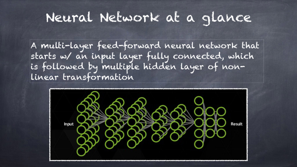
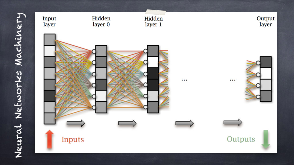
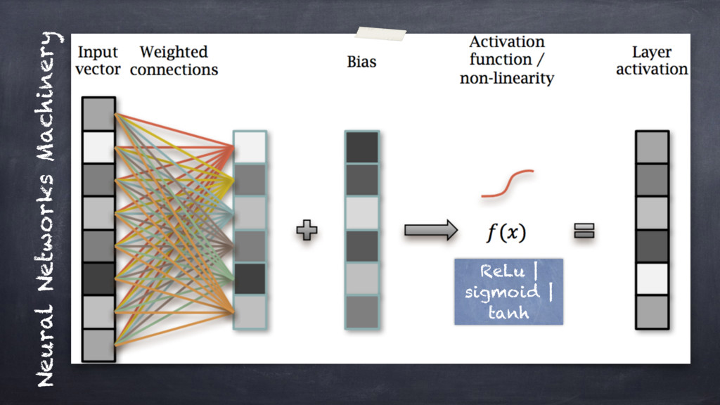
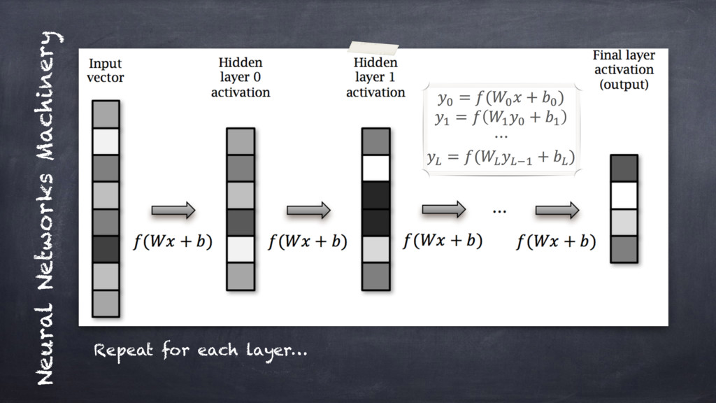
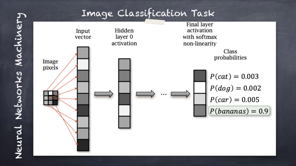
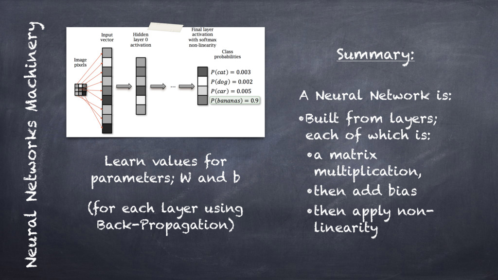
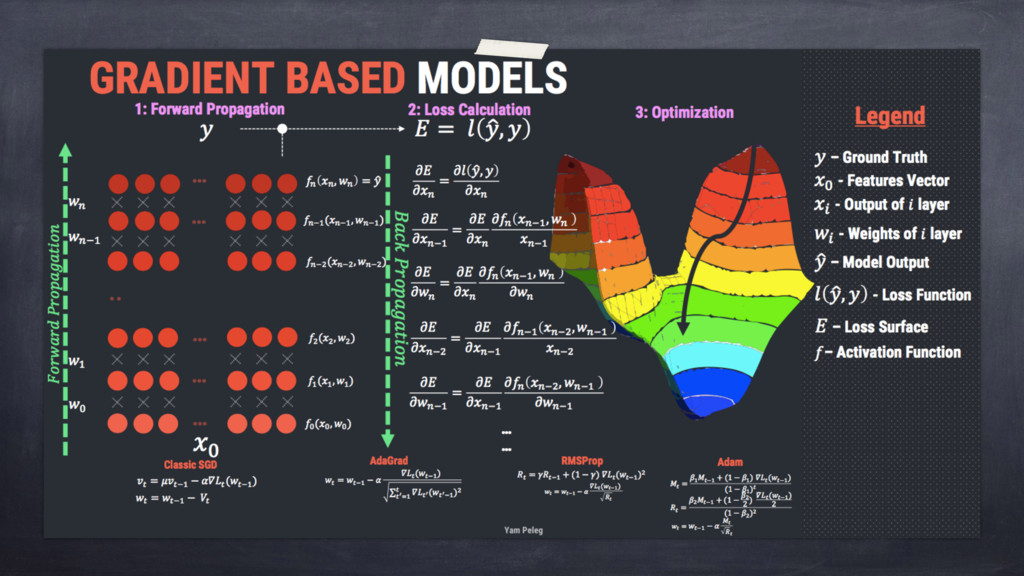
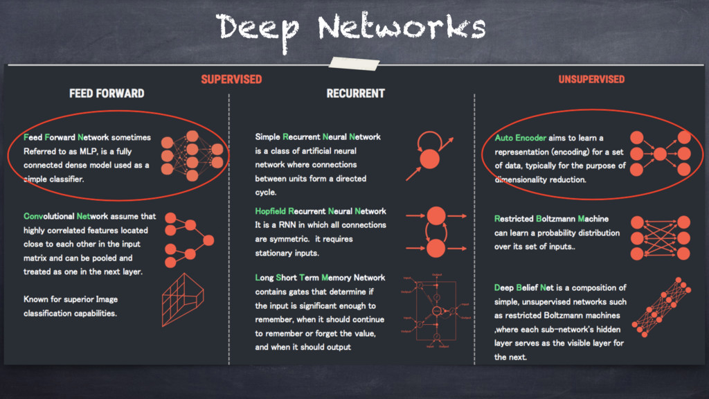
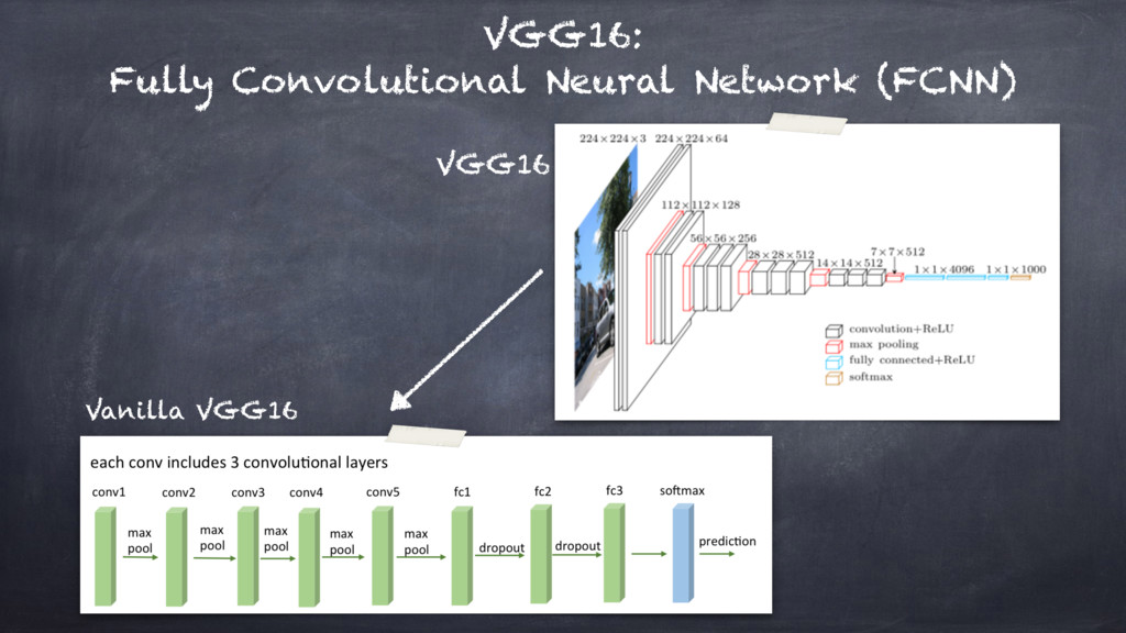
A classical introduction to the topic would go through explaining
about "activation functions", "optimisers & gradients", "batches", "feed-forward" and
"recurrent" multi-layer networks.
This is the "conventional" way: leveraging on a more theoretical perspective to ultimately explain how to
effectively implement Artificial Neural Networks (ANN).

The other way, namely the "unconventional way", to introduce Deep Learning
is from the perspective of the computational model it requires.
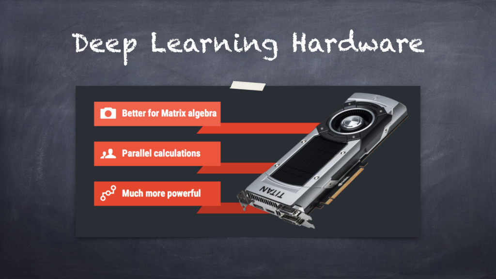
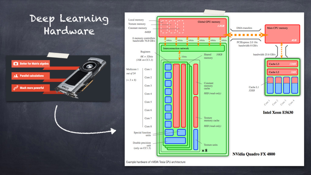
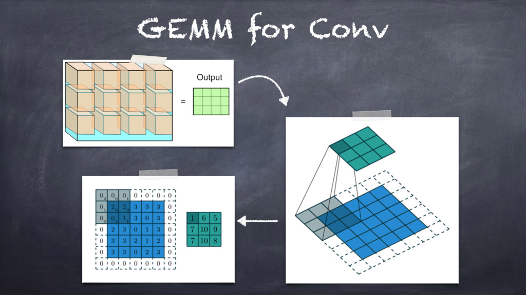
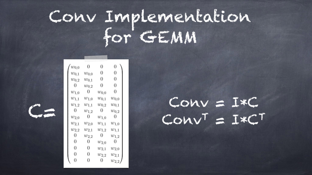
Therefore, this is the case when you may want to describe ANNs in terms of "Accelerated Kernel Matrix Multiplication" and
the gem[m|v] BLAS library, parallel execution models, and CPUs vs GPUs computing.
This is exactly the perspective I intend to pursue in this talk.

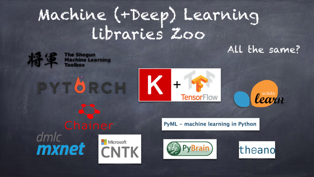
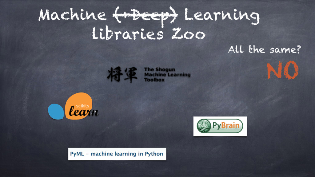
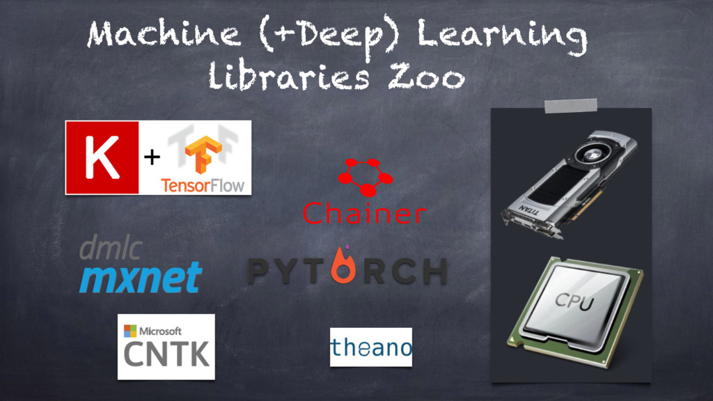
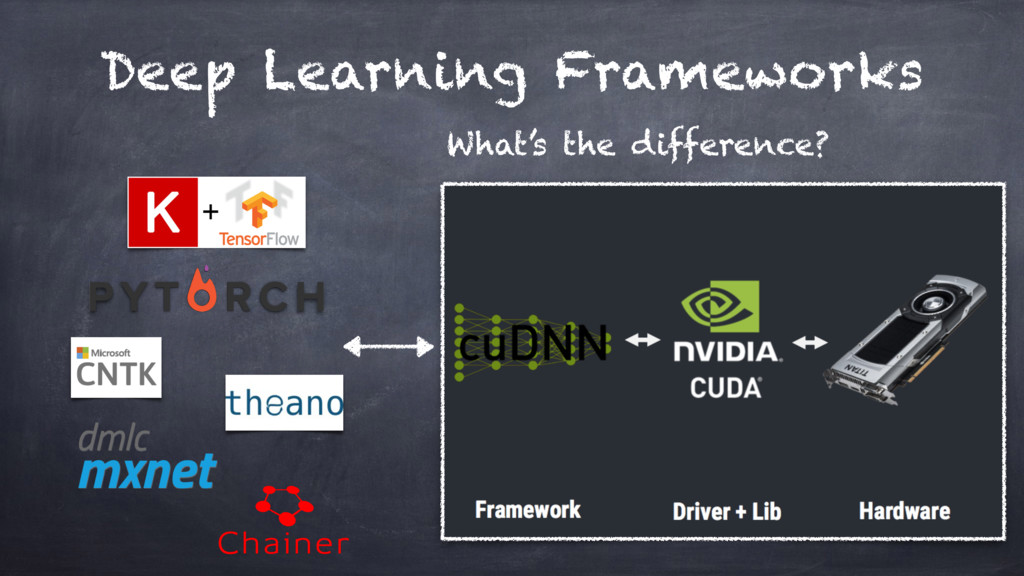
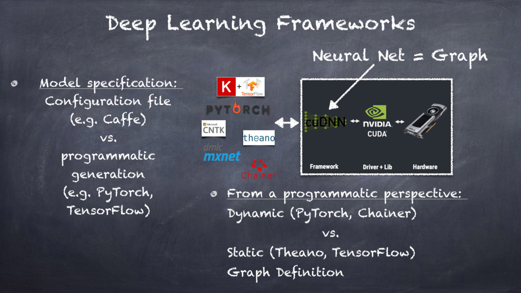
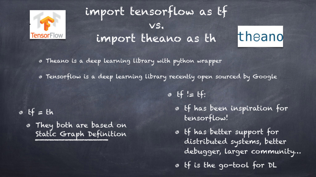
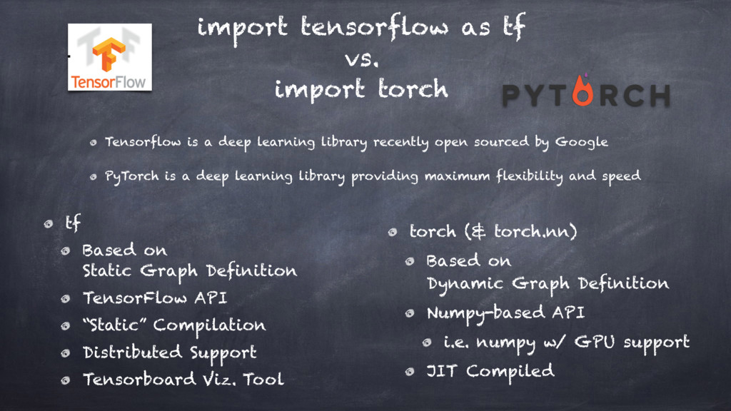
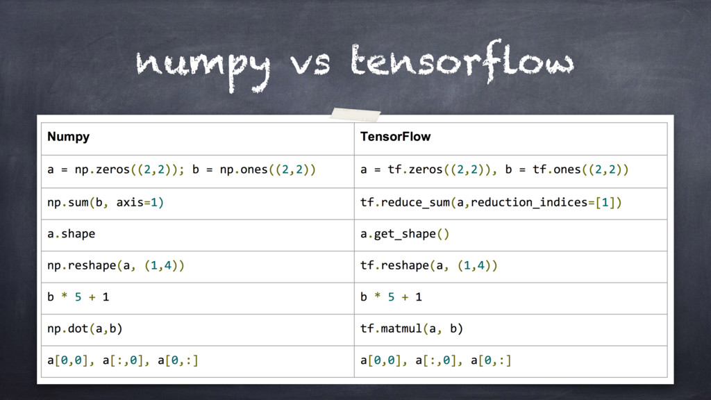
Different libraries and tools from the Python ecosystem, namely theano, tensorflow, and pytorch, will be presented
and compared, specifically in terms of their underlying computational models.

Transcript

1. Deep Learning The Unconventional Introduction Data Scientist and Researcher Fondazione Bruno Kessler (FBK)
 Trento, Italy Valerio Maggio @leriomaggio (in Python)
4. Hint:
 Doctor Who?
5. Quite Conventional Intro to 
 Deep Learning
7. A multi-layer feed-forward neural network that starts w/ an input layer fully connected, which is followed by multiple hidden layer of non- linear transformation Neural Network at a glance
9. Neural Networks Machinery
10. ReLu | sigmoid | tanh Neural Networks Machinery
11. Repeat for each layer… Neural Networks Machinery
12. Image Classification Task Neural Networks Machinery
13. Summary:
 
 A Neural Network is: •Built from layers; each of which is: •a matrix multiplication, •then add bias •then apply non- linearity Learn values for parameters; W and b (for each layer using Back-Propagation) Neural Networks Machinery
15. Deep Networks
17. Deep Learning is quite like the Tardis…
18. Deeply Wobbly, Timey Wimey… stuff
19. So, what about Python?
20. Machine (+Deep) Learning libraries Zoo All the same?
21. Machine (+Deep) Learning libraries Zoo NO All the same?
22. Machine (+Deep) Learning libraries Zoo
23. Deep Learning Hardware
24. Deep Learning Hardware
25. VGG16: 
 Fully Convolutional Neural Network (FCNN) Vanilla VGG16 VGG16
26. Source: J, Yangqing - Learning Semantic Image Representations at a Large Scale, University of California, Berkeley - 2014
27. GEneralised Matrix-to-Matrix Multiplication GEMM (BLAS l3) is at the heart of Deep Learning The difference is in the SCALE:
 A single layer in a typical network may require the multiplication of 256x1,152 matrix by 1,152x192 matrix —> 256x192 result. 
 Naively, that requires 57 million (256 x 1,152, x 192) floating point operations and there can be dozens of these layers in a modern architecture
28. Fully Connected (FC) Layer
29. Convolutional (Conv) Layer
30. GEMM for Conv
31. Conv Implementation 
 for GEMM C= Conv = I*C ConvT = I*CT
32. Deep Learning Frameworks What’s the difference?
33. Deep Learning Frameworks Model specification: 
 Configuration file 
 (e.g. Caffe) 
 vs. 
 programmatic generation 
 (e.g. PyTorch, 
 TensorFlow) From a programmatic perspective: 
 Dynamic (PyTorch, Chainer) 
 vs. 
 Static (Theano, TensorFlow) 
 Graph Definition Neural Net = Graph
34. import tensorflow as tf vs. import theano as th Theano is a deep learning library with python wrapper Tensorflow is a deep learning library recently open sourced by Google tf = th They both are based on 
 Static Graph Definition
 
 
 tf != tf: tf has been inspiration for tensorflow! tf has better support for distributed systems, better debugger, larger community… tf is the go-tool for DL
35. import tensorflow as tf vs. import torch Tensorflow is a deep learning library recently open sourced by Google PyTorch is a deep learning library providing maximum flexibility and speed tf Based on 
 Static Graph Definition TensorFlow API “Static” Compilation Distributed Support Tensorboard Viz. Tool torch (& torch.nn) Based on 
 Dynamic Graph Definition Numpy-based API i.e. numpy w/ GPU support JIT Compiled
36. Focus on
37. What does 
 TensorFlow provides? TensorFlow provides primitives for defining functions on tensors and automatically computing their derivatives
38. Tensor?
39. Tensor? from: Matthew Rocklin (@mrocklin), 
 Lead Data Scientist @ Continuum Analytics
40. Tensor? An intuitive way to represent a tensor is a
 multidimensional array from: Matthew Rocklin (@mrocklin), 
 Lead Data Scientist @ Continuum Analytics
41. numpy vs tensorflow
42. tf requires explicit evaluation (i.e. symbolic computation) >>> import numpy as np >>> import tensorflow as tf >>> a = np.zeros((2,2) >>> print(a) [[ 0. 0.] [ 0. 0.]] >>> ta = tf.zeros((2,2)) >>> print(ta) Tensor("zeros_1:0", shape=(2, 2), dtype=float32) >>> print(ta.eval()) [[ 0. 0.] [ 0. 0.]]
43. tf.Graph (IDEA) A Machine Learning application is the result of the repeated computation of complex mathematical expressions, thus we could describe this computation by using a Data Flow Graph Data Flow Graph: each Node represents the instance of a mathematical operation:
 multiply, add, divide each Edge is a multi-dimensional data set (tensors) on which the operations are performed.
44. tf.Graph Node: instantiation of an operation w/ inputs (>= 2), outputs >= 0.
 Data Edges: 
 carriers tensors, where an output of one operation (from one node) becomes the input for another operation.
 Dependency Edges: 
 control dependency between two nodes (i.e. "happens before" relationship). Before and after graph transformation for partial execution
45. Logistic Regression
46. source: https:/ /github.com/tensorflow/fold tf.Graph w/ multi-layers
47. Logistic Neuron MNIST Dataset 28x28 B/W Images
48. Logistic Neuron: #1 Model >>> import tensorflow as tf >>> #tf Graph Input >>> x = tf.placeholder("float", [None, 784]). # 784 = 28 x 28 >>> y = tf.placeholder("float", [None, 10])
 >>> with tf.name_scope("model") as scope: # Set model weights W = tf.Variable(tf.zeros([dims, nb_classes])) b = tf.Variable(tf.zeros([nb_classes])) activation = tf.nn.softmax(tf.matmul(x, W) + b) # Softmax
 # Add summary ops to collect data w_h = tf.summary.histogram("weights_histogram", W) b_h = tf.summary.histogram("biases_histograms", b) tf.summary.scalar('mean_weights', tf.reduce_mean(W)) tf.summary.scalar(‘mean_bias’, tf.reduce_mean(b)) Repeat this for each layer you want to add
49. Logistic Neuron: #2 Cost Function & Train >>> #Minimize error using cross entropy >>> #Note: More name scopes will clean up graph representation >>> with tf.name_scope("cost_function") as scope: cross_entropy = y*tf.log(activation) cost = tf.reduce_mean(-tf.reduce_sum(cross_entropy,reduction_indices=1)) #Create a summary to monitor the cost function tf.summary.scalar("cost_function", cost) tf.summary.histogram("cost_histogram", cost) >>> with tf.name_scope("train") as scope: #Set the Optimizer learning_rate = 0.01 optimizer = tf.train.GradientDescentOptimizer(learning_rate).minimize(cost)
50. Logistic Neuron: #3 Metrics & Summaries >>> with tf.name_scope('accuracy') as scope: correct_prediction = tf.equal(tf.argmax(activation, 1), tf.argmax(y, 1)) #Calculate accuracy accuracy = tf.reduce_mean(tf.cast(correct_prediction, "float")) #Create a summary to monitor the cost function t.f.summary.scalar("accuracy", accuracy)
 >>> #Plug TensorBoard Visualisation >>> writer = tf.summary.FileWriter(“/tmp/logistic_logs”, graph=tf.get_default_graph())
 >>> for var in tf.get_collection(tf.GraphKeys.SUMMARIES): … print(var.name, end=‘, ’)
 model/weights_histogram:0, model/biases_histograms:0, model/mean_weights:0, model/mean_bias:0, cost_function/cost_function:0, cost_function/cost_histogram:0, accuracy/accuracy:0 >>> summary_op = tf.summary.merge_all() >>> print('Summary Op: ', summary_op) Summary Op: Tensor("Merge_1/MergeSummary:0", shape=(), dtype=string)
51. >>> # Launch the graph >>> with tf.Session() as session: # Initializing the variables session.run(tf.global_variables_initializer()) cost_epochs = [] # Training cycle for epoch in range(training_epochs): _, summary, c = session.run(fetches=[optimizer, summary_op, cost], feed_dict={x: X_train, y: Y_train}) cost_epochs.append(c) writer.add_summary(summary=summary, global_step=epoch) Logistic Neuron: #4 Learning Loop
52. >>> # Launch the graph >>> with tf.Session() as session: # Initializing the variables session.run(tf.global_variables_initializer()) cost_epochs = [] # Training cycle for epoch in range(training_epochs): _, summary, c = session.run(fetches=[optimizer, summary_op, cost], feed_dict={x: X_train, y: Y_train}) cost_epochs.append(c) writer.add_summary(summary=summary, global_step=epoch) >>> #plotting >>> plt.plot(range(len(cost_epochs)), cost_epochs, 'o', … label='Logistic Regression Training phase’) >>> plt.show() Logistic Neuron: #4 Learning Loop
53. Tensorboard
54. Tensorboard: Scalars
55. Tensorboard: Graph
56. Tensorboard: Histograms
57. (Quick) 
 Look at Keras (http:/ /keras.io)
58. Keras Keras is a high-level neural networks API, written in Python and capable of running on top of TensorFlow, CNTK, or Theano (and mxNet). Keras: allows for easy and fast prototyping (through user friendliness, modularity, and extensibility). supports both convolutional networks and recurrent networks, as well as combinations of the two. runs seamlessly on CPU and GPU. Keras is compatible with: Python 2.7 - 3.5 from tf.contrib import keras (soon) from tf import keras The Deep Learning library for perfectionist, with deadlines
59. Logistic Neuron using Keras >>> from keras.models import Sequential >>> from keras.layers import Dense, Activation
 >>> model = Sequential() >>> model.add(Dense(10, input_shape=(784,), …. activation=‘sigmoid’)) >>> model.add(Activation(‘softmax')) >>> model.compile(optimizer='sgd', … loss=‘categorical_crossentropy’) >>> model.fit(X_train, Y_train, epochs=25) Epoch 1/10 61878/61878 [==============================] - 5s - loss: 1.9928 Epoch 2/10 61878/61878 [==============================] - 4s - loss: 1.8417 Epoch 3/10 61878/61878 [==============================] - 4s - loss: 1.7851 Epoch 4/10 61878/61878 [==============================] - 4s - loss: 1.7492 Epoch 5/10 61878/61878 [==============================] - 4s - loss: 1.7235 Epoch 6/10 61878/61878 [==============================] - 4s - loss: 1.7040 Epoch 7/10 61878/61878 [==============================] - 4s - loss: 1.6886 Epoch 8/10 61878/61878 [==============================] - 4s - loss: 1.6762 Epoch 9/10 61878/61878 [==============================] - 4s - loss: 1.6661 Epoch 10/10 61878/61878 [==============================] - 4s - loss: 1.6577
60. Deep Learning with 
 Keras and TensorFlow Tutorial:
 
 https:/ /github.com/leriomaggio/ deep-learning-keras-tensorflow
61. Thank you! @leriomaggio