Convex Optimization with Abstract Linear Operators

Source - http://www.icassp2016.org/ShowRecording.asp?C=0316DAB2

Stephen P. Boyd - Stanford University

Convex Optimization with Abstract Linear Operators

Tuesday 22 March 2016, 10.20 - 11.10 (Grand Ballroom II & III)

Transcript

1. Convex Optimization with Abstract Linear Operators Stephen Boyd and Steven Diamond EE & CS Departments Stanford University ICASSP, Shanghai, March 22 2016 1
2. Outline Convex Optimization Examples Matrix-Free Methods Summary 2
3. Outline Convex Optimization Examples Matrix-Free Methods Summary Convex Optimization 3
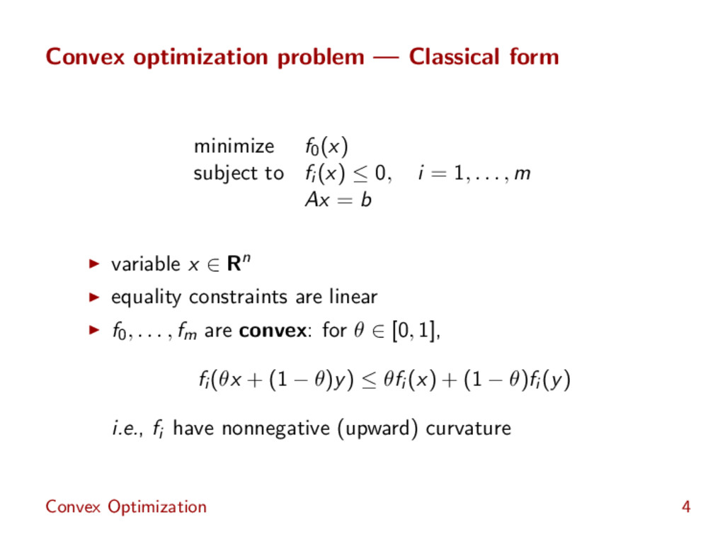
4. Convex optimization problem — Classical form minimize f0(x) subject to fi (x) ≤ 0, i = 1, . . . , m Ax = b variable x ∈ Rn equality constraints are linear f0, . . . , fm are convex: for θ ∈ [0, 1], fi (θx + (1 − θ)y) ≤ θfi (x) + (1 − θ)fi (y) i.e., fi have nonnegative (upward) curvature Convex Optimization 4
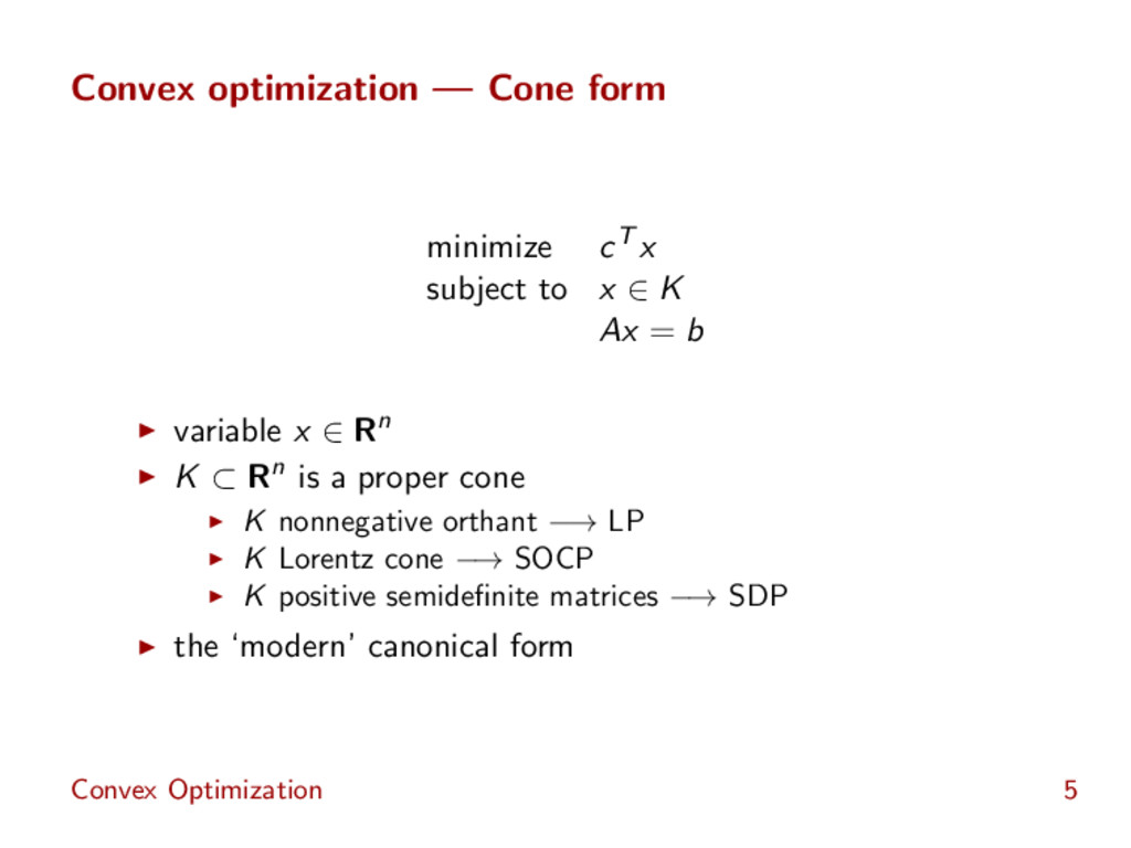
5. Convex optimization — Cone form minimize cT x subject to x ∈ K Ax = b variable x ∈ Rn K ⊂ Rn is a proper cone K nonnegative orthant −→ LP K Lorentz cone −→ SOCP K positive semidefinite matrices −→ SDP the ‘modern’ canonical form Convex Optimization 5
6. Why beautiful, nearly complete theory duality, optimality conditions, . . . Convex Optimization 6
7. Why beautiful, nearly complete theory duality, optimality conditions, . . . effective algorithms, methods (in theory and practice) get global solution (and optimality certificate) polynomial complexity Convex Optimization 6
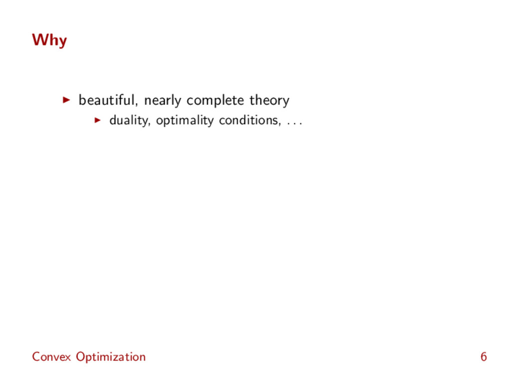
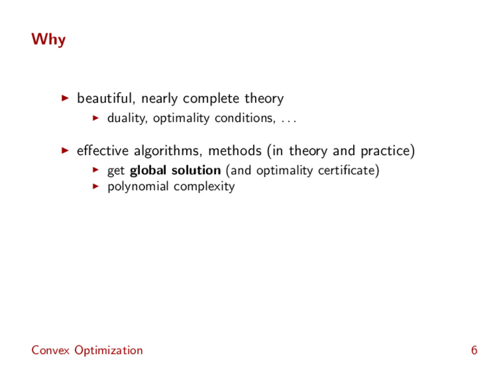
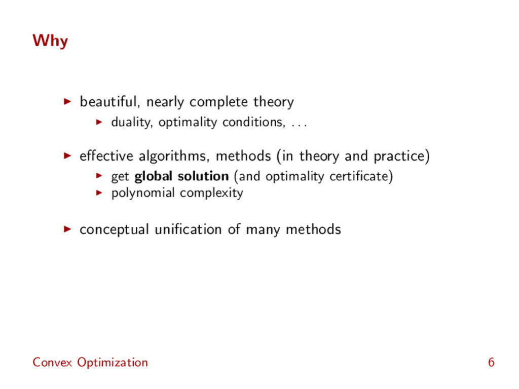
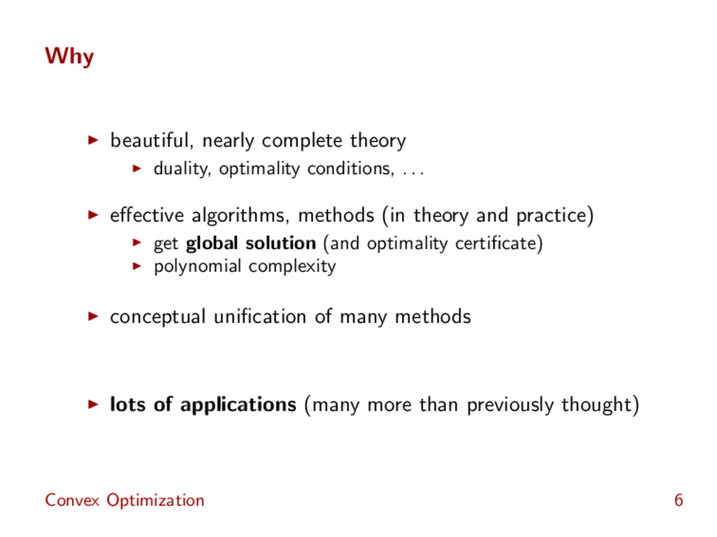
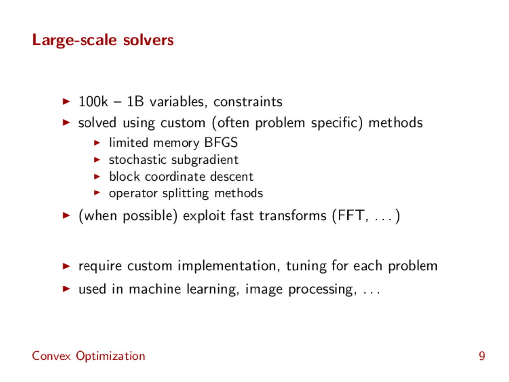
8. Why beautiful, nearly complete theory duality, optimality conditions, . . . effective algorithms, methods (in theory and practice) get global solution (and optimality certificate) polynomial complexity conceptual unification of many methods Convex Optimization 6
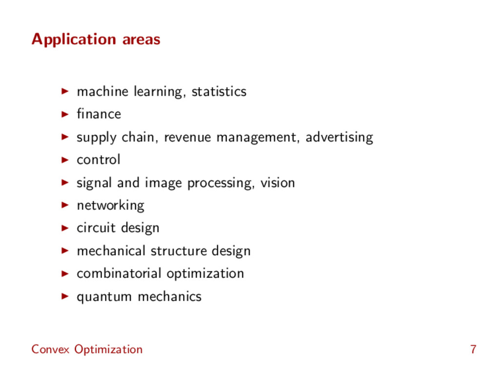
9. Why beautiful, nearly complete theory duality, optimality conditions, . . . effective algorithms, methods (in theory and practice) get global solution (and optimality certificate) polynomial complexity conceptual unification of many methods lots of applications (many more than previously thought) Convex Optimization 6
10. Application areas machine learning, statistics finance supply chain, revenue management, advertising control signal and image processing, vision networking circuit design mechanical structure design combinatorial optimization quantum mechanics Convex Optimization 7
11. Medium-scale solvers 1000s–10000s variables, constraints reliably solved by interior-point methods on single machine (especially for problems in standard cone form) exploit problem sparsity Convex Optimization 8
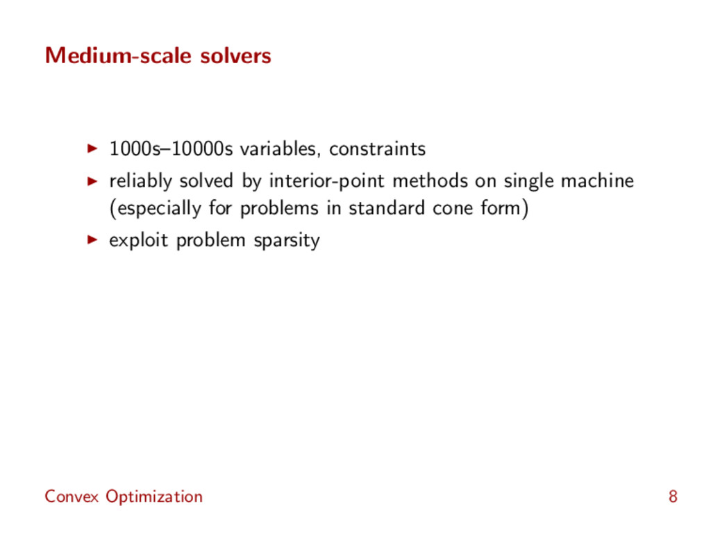
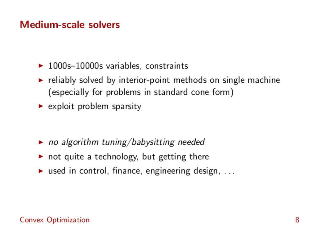
12. Medium-scale solvers 1000s–10000s variables, constraints reliably solved by interior-point methods on single machine (especially for problems in standard cone form) exploit problem sparsity no algorithm tuning/babysitting needed not quite a technology, but getting there used in control, finance, engineering design, . . . Convex Optimization 8
13. Large-scale solvers 100k – 1B variables, constraints solved using custom (often problem specific) methods limited memory BFGS stochastic subgradient block coordinate descent operator splitting methods (when possible) exploit fast transforms (FFT, . . . ) require custom implementation, tuning for each problem used in machine learning, image processing, . . . Convex Optimization 9
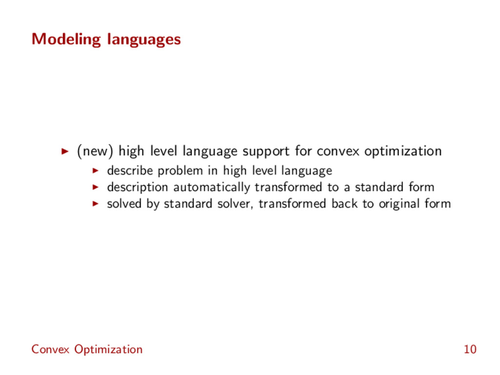
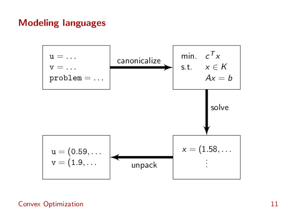
14. Modeling languages (new) high level language support for convex optimization describe problem in high level language description automatically transformed to a standard form solved by standard solver, transformed back to original form Convex Optimization 10
15. Modeling languages u = . . . v = . . . problem = . . . min. cT x s.t. x ∈ K Ax = b x = (1.58, . . . . . . u = (0.59, . . . v = (1.9, . . . canonicalize solve unpack Convex Optimization 11
16. Implementations convex optimization modeling language implementations YALMIP, CVX (Matlab) CVXPY (Python) Convex.jl (Julia) widely used for applications with medium scale problems Convex Optimization 12
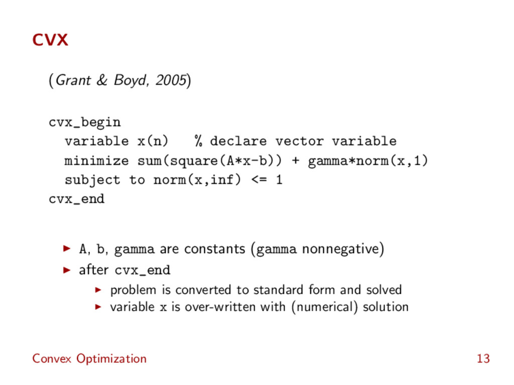
17. CVX (Grant & Boyd, 2005) cvx_begin variable x(n) % declare vector variable minimize sum(square(A*x-b)) + gamma*norm(x,1) subject to norm(x,inf) <= 1 cvx_end A, b, gamma are constants (gamma nonnegative) after cvx_end problem is converted to standard form and solved variable x is over-written with (numerical) solution Convex Optimization 13
18. CVXPY (Diamond & Boyd, 2013) from cvxpy import * x = Variable(n) cost = norm(A*x-b) + gamma*norm(x,1) prob = Problem(Minimize(cost), [norm(x,"inf") <= 1]) opt_val = prob.solve() solution = x.value A, b, gamma are constants (gamma nonnegative) solve method converts problem to standard form, solves, assigns value attributes Convex Optimization 14
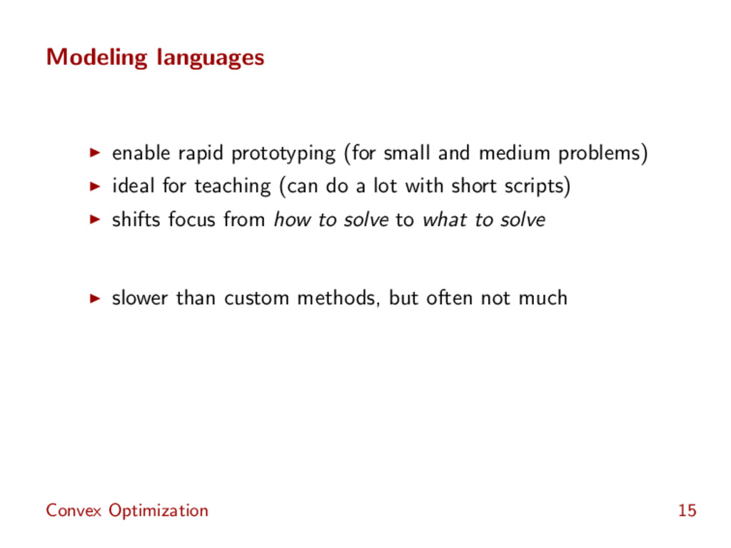
19. Modeling languages enable rapid prototyping (for small and medium problems) ideal for teaching (can do a lot with short scripts) shifts focus from how to solve to what to solve slower than custom methods, but often not much Convex Optimization 15
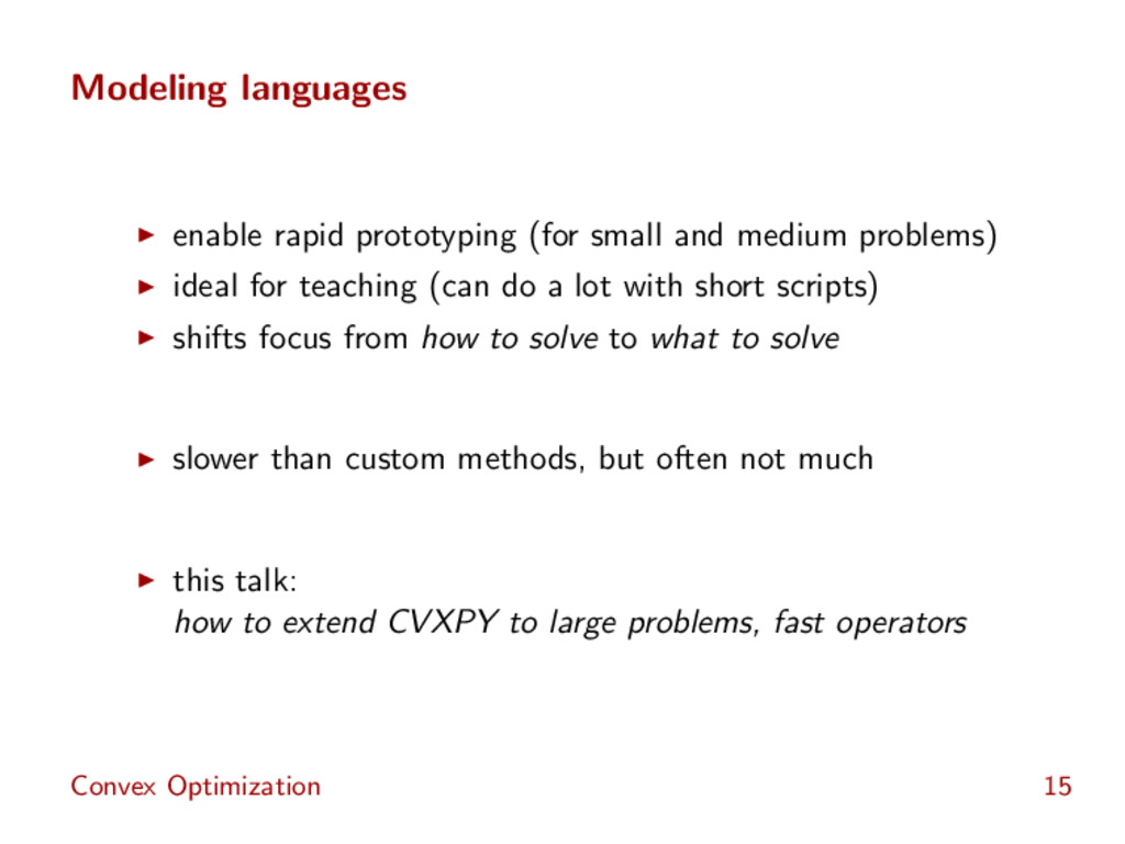
20. Modeling languages enable rapid prototyping (for small and medium problems) ideal for teaching (can do a lot with short scripts) shifts focus from how to solve to what to solve slower than custom methods, but often not much this talk: how to extend CVXPY to large problems, fast operators Convex Optimization 15
21. Outline Convex Optimization Examples Matrix-Free Methods Summary Examples 16
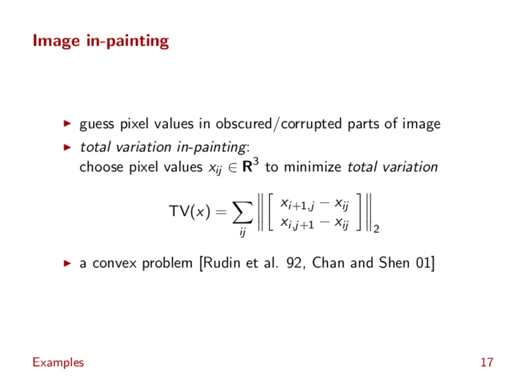
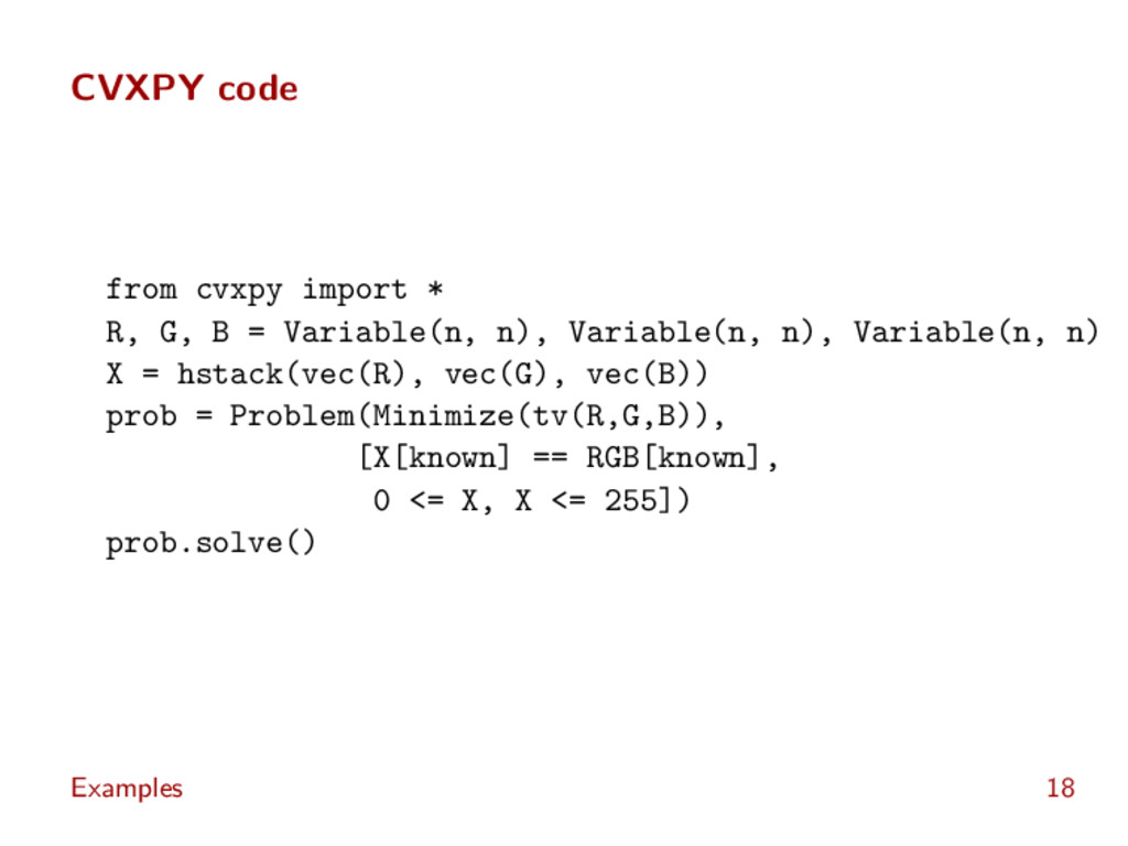
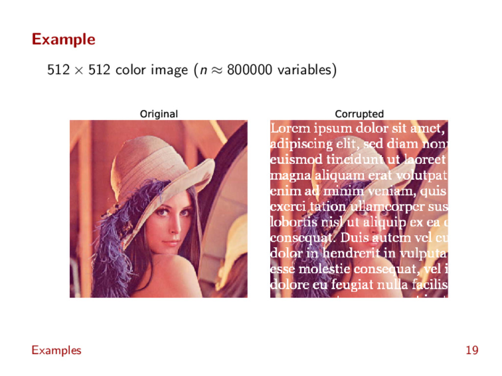
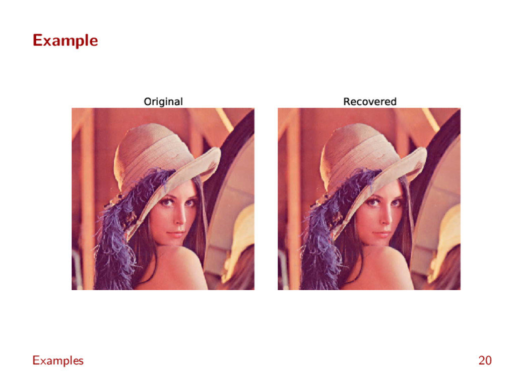
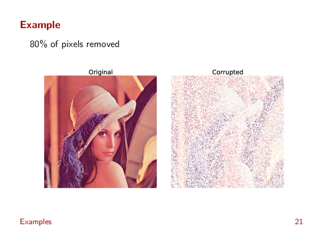
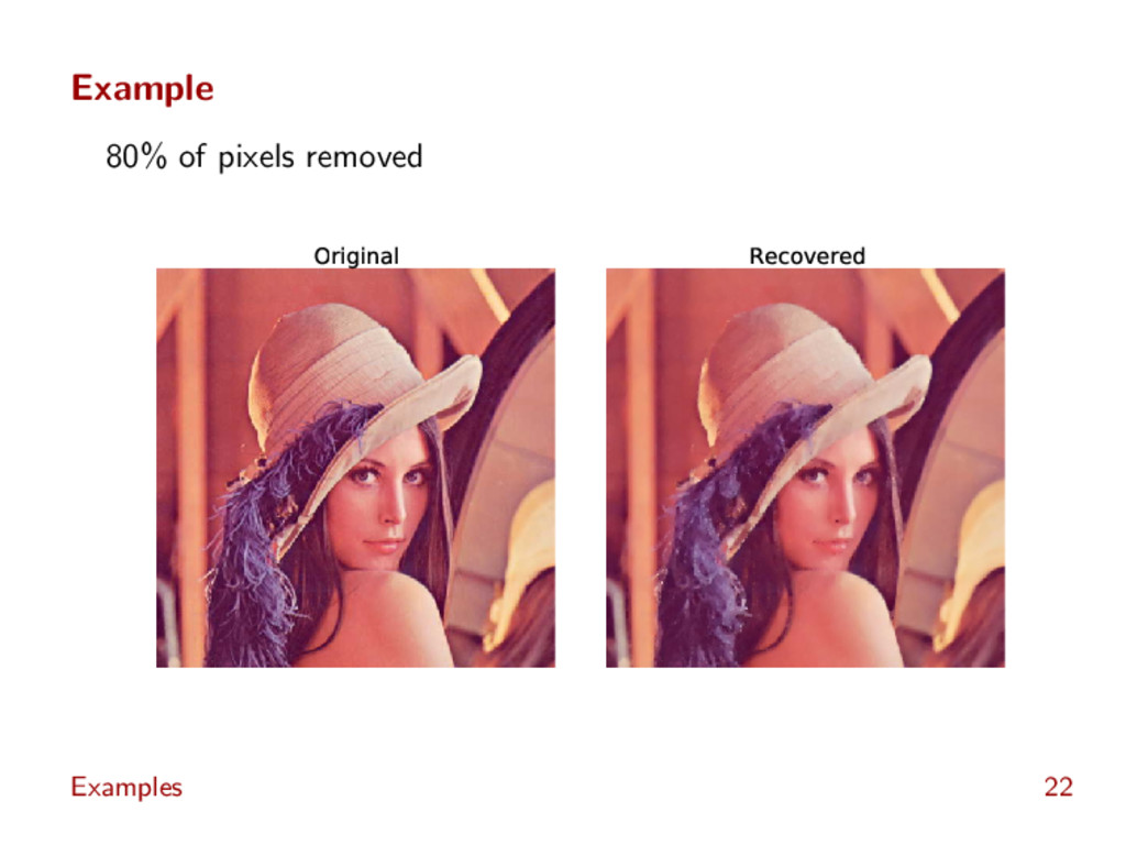
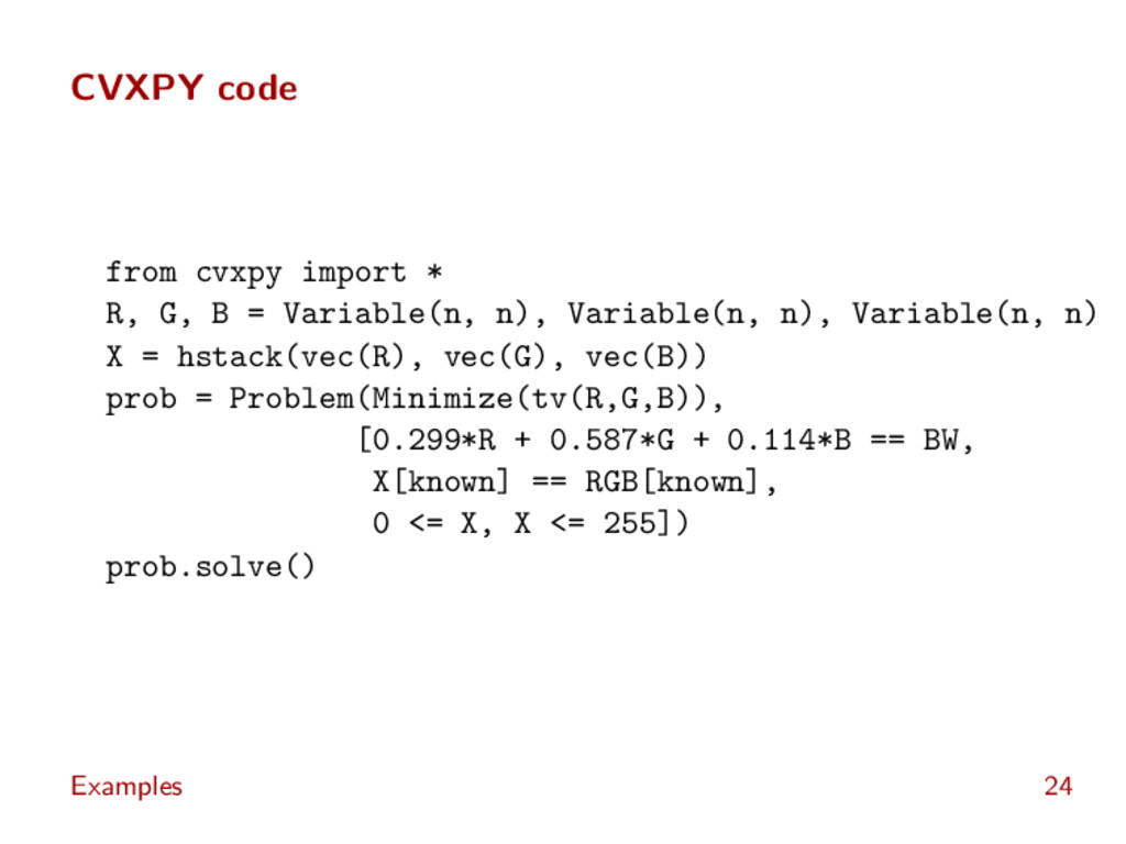
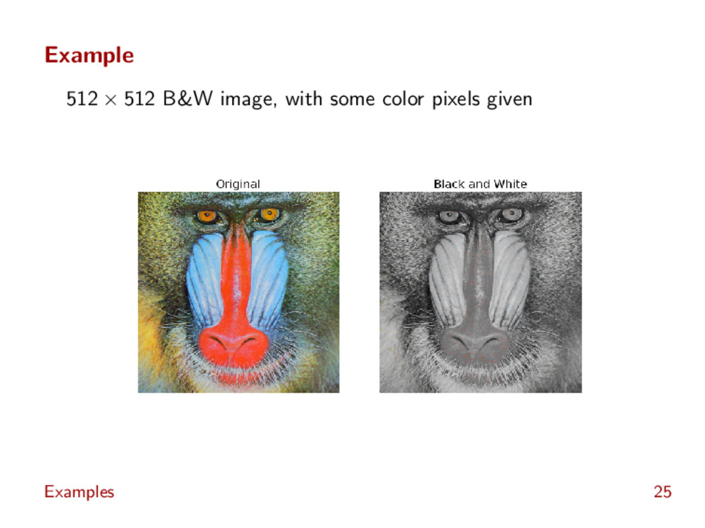
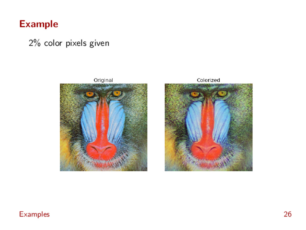
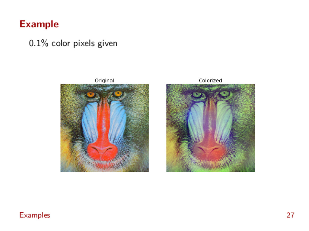
22. Image in-painting guess pixel values in obscured/corrupted parts of image total variation in-painting: choose pixel values xij ∈ R3 to minimize total variation TV(x) = ij xi+1,j − xij xi,j+1 − xij 2 a convex problem [Rudin et al. 92, Chan and Shen 01] Examples 17
23. CVXPY code from cvxpy import * R, G, B = Variable(n, n), Variable(n, n), Variable(n, n) X = hstack(vec(R), vec(G), vec(B)) prob = Problem(Minimize(tv(R,G,B)), [X[known] == RGB[known], 0 <= X, X <= 255]) prob.solve() Examples 18
24. Example 512 × 512 color image (n ≈ 800000 variables) Original Corrupted Examples 19
25. Example Original Recovered Examples 20
26. Example 80% of pixels removed Original Corrupted Examples 21
27. Example 80% of pixels removed Original Recovered Examples 22
28. Colorization given B&W (scalar) pixel values, and a few colored pixels choose color pixel values xij ∈ R3 to minimize TV(x) subject to given B&W values a convex problem [Blomgren and Chan 98] Examples 23
29. CVXPY code from cvxpy import * R, G, B = Variable(n, n), Variable(n, n), Variable(n, n) X = hstack(vec(R), vec(G), vec(B)) prob = Problem(Minimize(tv(R,G,B)), [0.299*R + 0.587*G + 0.114*B == BW, X[known] == RGB[known], 0 <= X, X <= 255]) prob.solve() Examples 24
30. Example 512 × 512 B&W image, with some color pixels given Examples 25
31. Example 2% color pixels given Examples 26
32. Example 0.1% color pixels given Examples 27
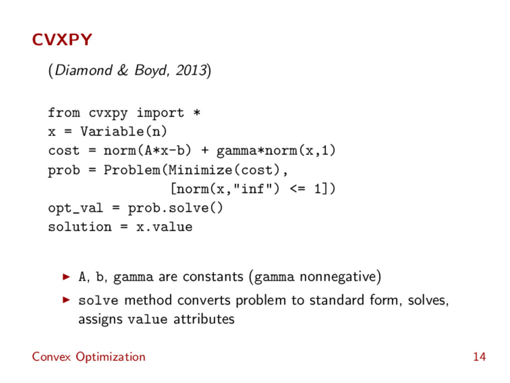
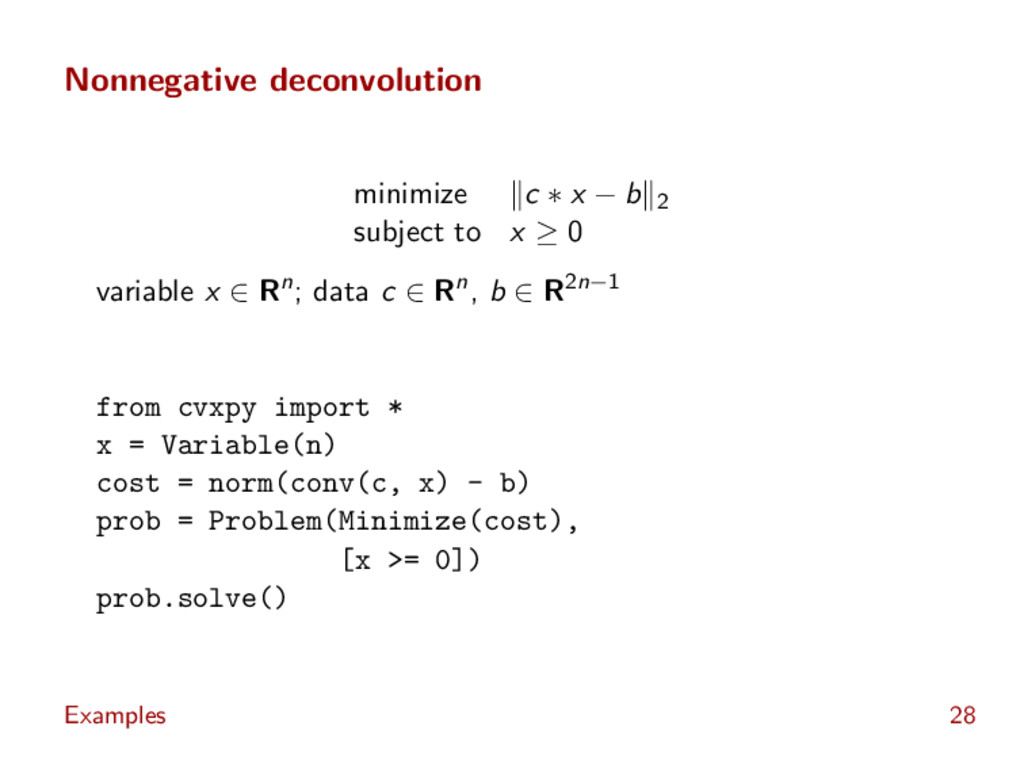
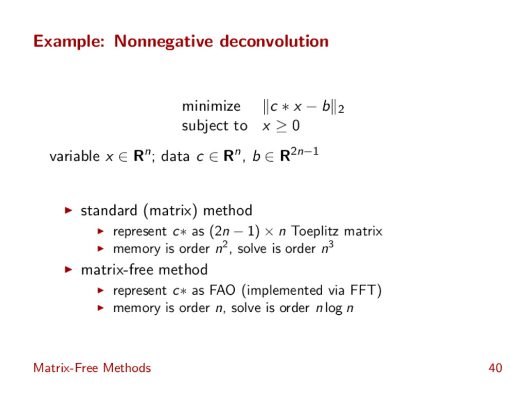
33. Nonnegative deconvolution minimize c ∗ x − b 2 subject to x ≥ 0 variable x ∈ Rn; data c ∈ Rn, b ∈ R2n−1 from cvxpy import * x = Variable(n) cost = norm(conv(c, x) - b) prob = Problem(Minimize(cost), [x >= 0]) prob.solve() Examples 28
34. Example Examples 29
35. Example Examples 30
36. Outline Convex Optimization Examples Matrix-Free Methods Summary Matrix-Free Methods 31
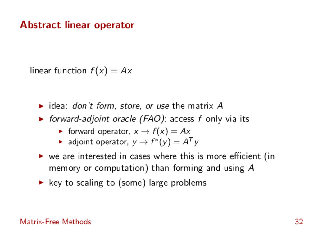
37. Abstract linear operator linear function f (x) = Ax idea: don’t form, store, or use the matrix A forward-adjoint oracle (FAO): access f only via its forward operator, x → f (x) = Ax adjoint operator, y → f ∗(y) = AT y we are interested in cases where this is more efficient (in memory or computation) than forming and using A key to scaling to (some) large problems Matrix-Free Methods 32
38. Examples of FAOs convolution, DFT O(n log n) Gauss, Wavelet, and other transforms O(n) Lyapunov, Sylvester mappings X → AXB O(n1.5) sparse matrix multiply O(nnz(A)) inverse of sparse triangular matrix O(nnz(A)) Matrix-Free Methods 33
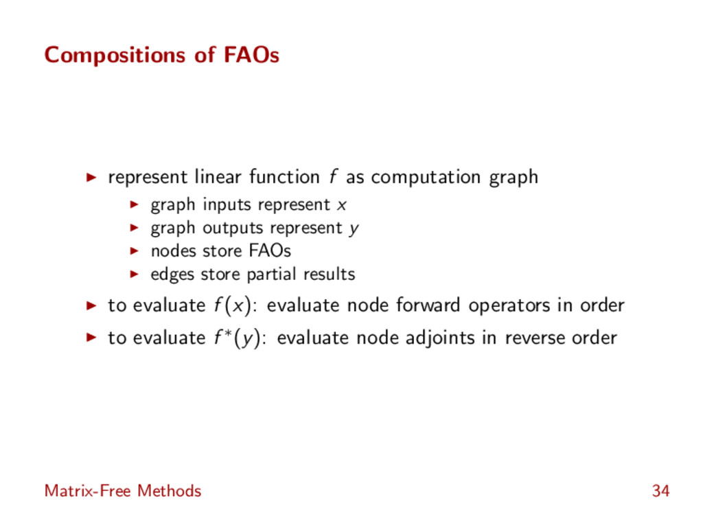
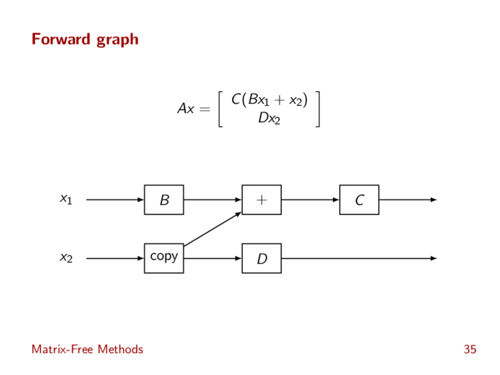
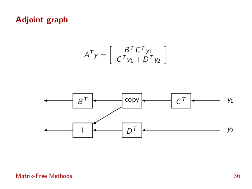
39. Compositions of FAOs represent linear function f as computation graph graph inputs represent x graph outputs represent y nodes store FAOs edges store partial results to evaluate f (x): evaluate node forward operators in order to evaluate f ∗(y): evaluate node adjoints in reverse order Matrix-Free Methods 34
40. Forward graph Ax = C(Bx1 + x2) Dx2 x1 x2 B copy + C D Matrix-Free Methods 35
41. Adjoint graph AT y = BT CT y1 CT y1 + DT y2 BT + copy CT DT y1 y2 Matrix-Free Methods 36
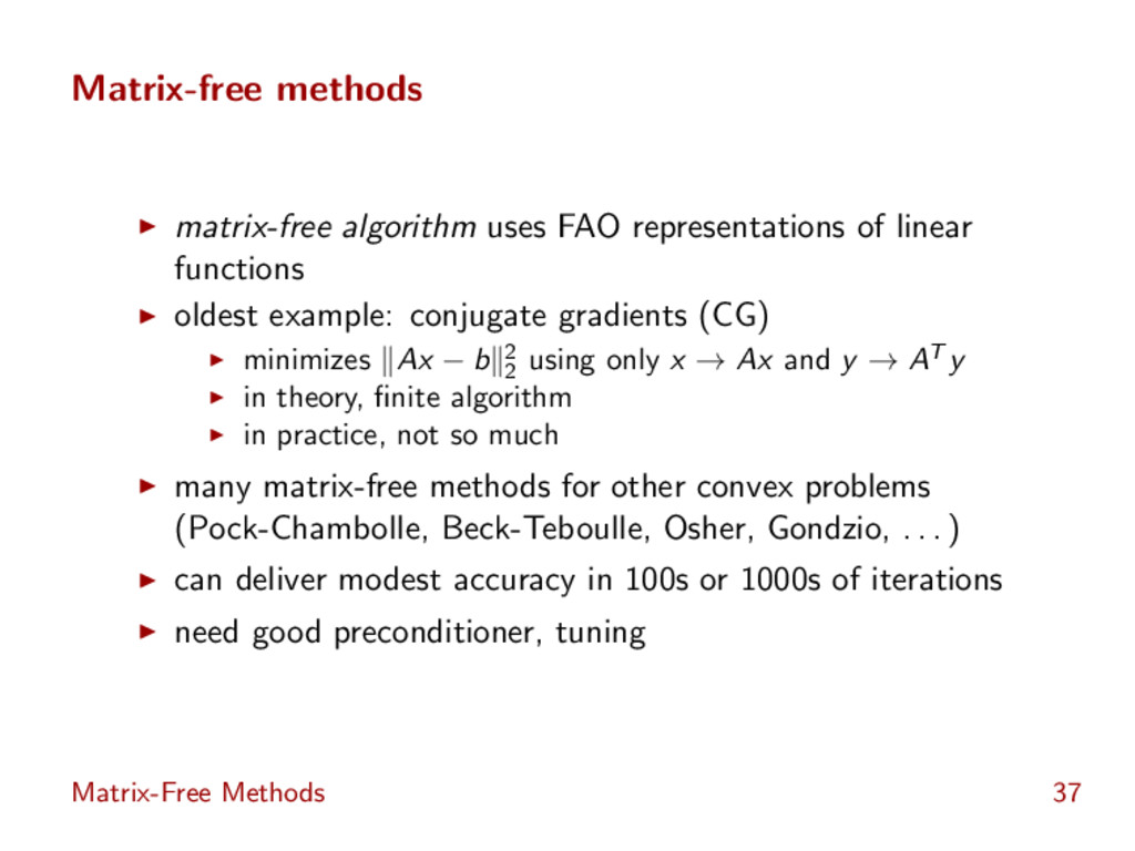
42. Matrix-free methods matrix-free algorithm uses FAO representations of linear functions oldest example: conjugate gradients (CG) minimizes Ax − b 2 2 using only x → Ax and y → AT y in theory, finite algorithm in practice, not so much many matrix-free methods for other convex problems (Pock-Chambolle, Beck-Teboulle, Osher, Gondzio, . . . ) can deliver modest accuracy in 100s or 1000s of iterations need good preconditioner, tuning Matrix-Free Methods 37
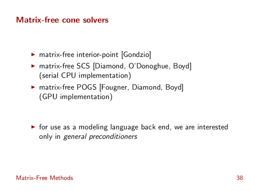
43. Matrix-free cone solvers matrix-free interior-point [Gondzio] matrix-free SCS [Diamond, O’Donoghue, Boyd] (serial CPU implementation) matrix-free POGS [Fougner, Diamond, Boyd] (GPU implementation) for use as a modeling language back end, we are interested only in general preconditioners Matrix-Free Methods 38
44. Matrix-free CVXPY preliminary version [Diamond] canonicalizes to a matrix-free cone program solves using matrix-free SCS or POGS Matrix-Free Methods 39
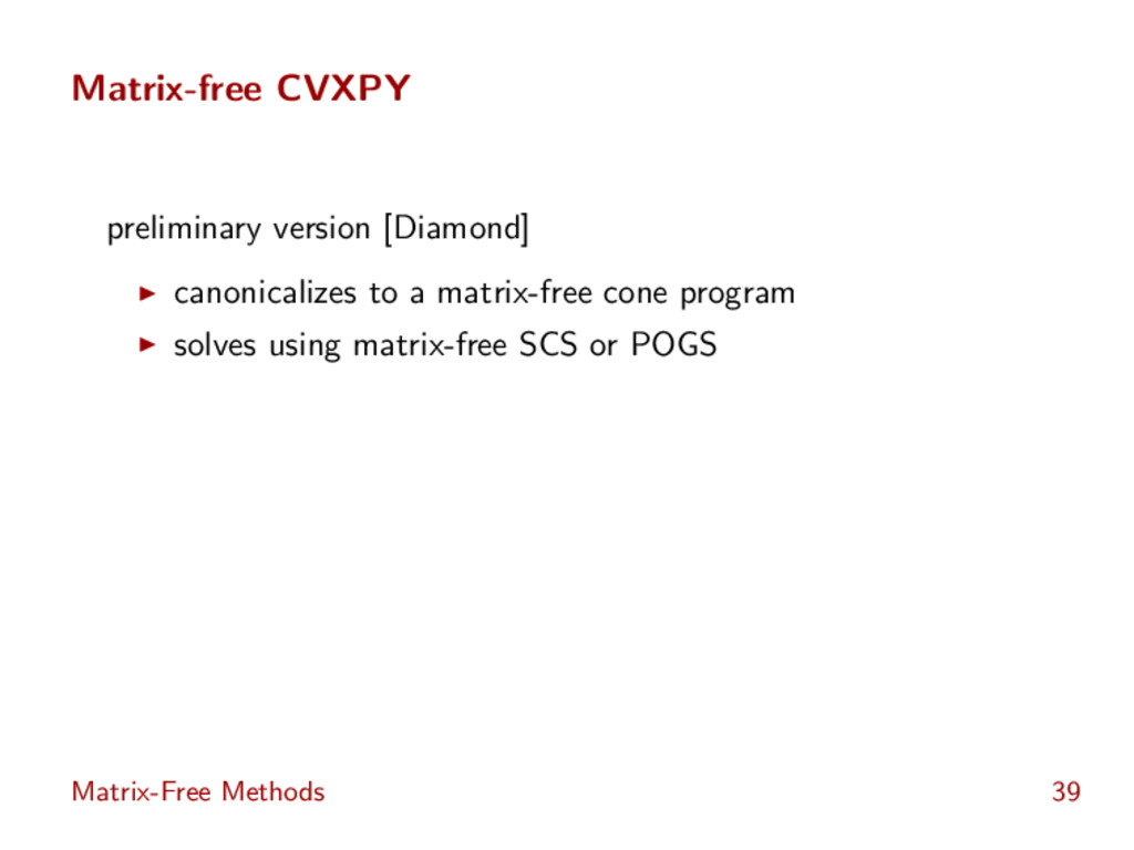
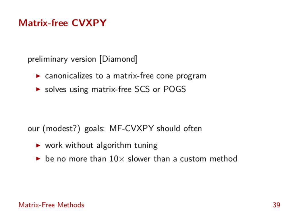
45. Matrix-free CVXPY preliminary version [Diamond] canonicalizes to a matrix-free cone program solves using matrix-free SCS or POGS our (modest?) goals: MF-CVXPY should often work without algorithm tuning be no more than 10× slower than a custom method Matrix-Free Methods 39
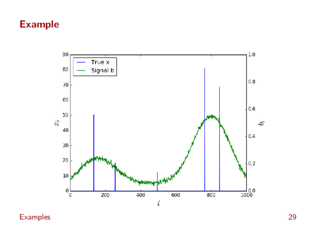
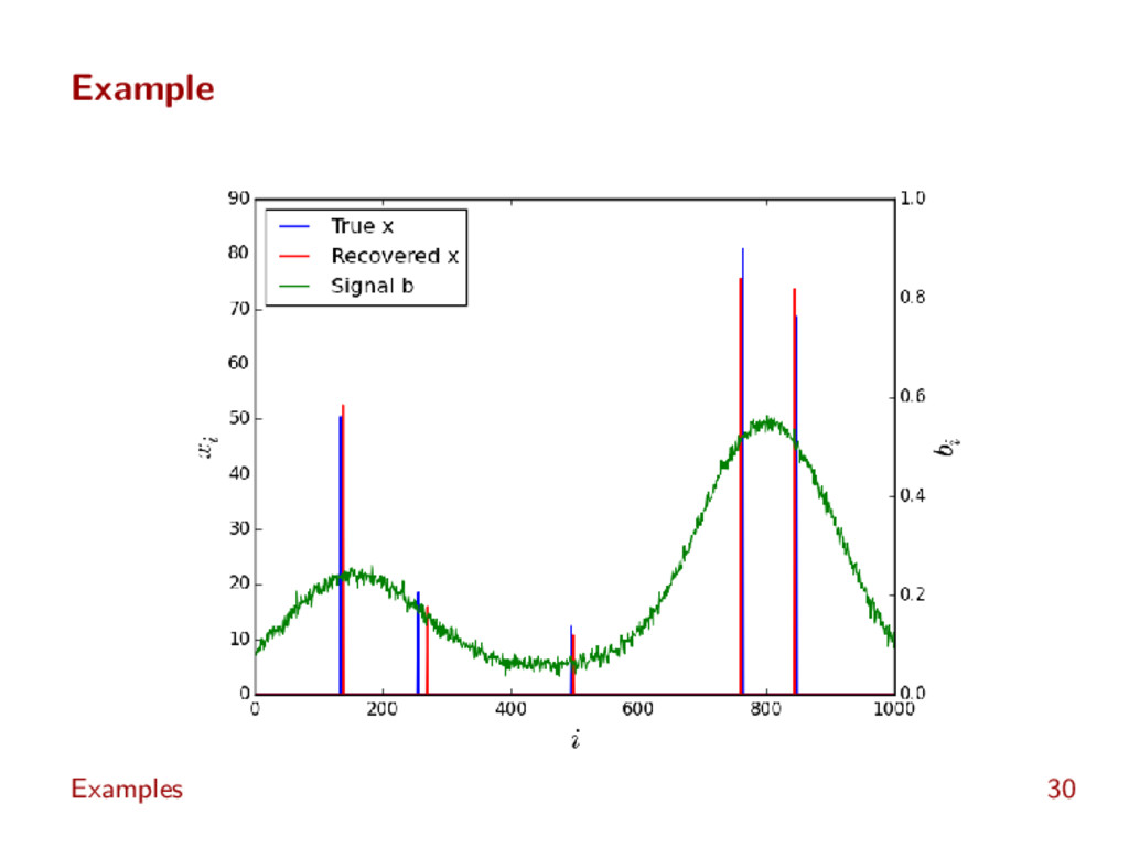
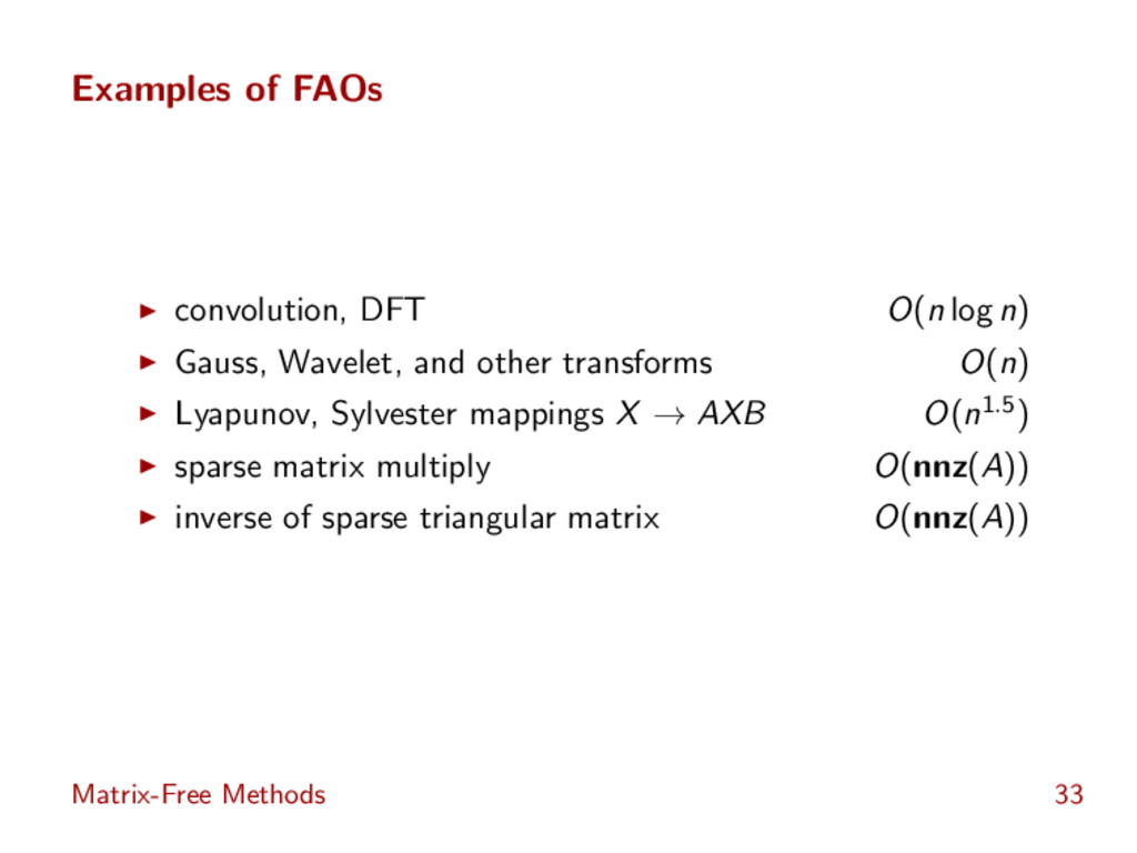
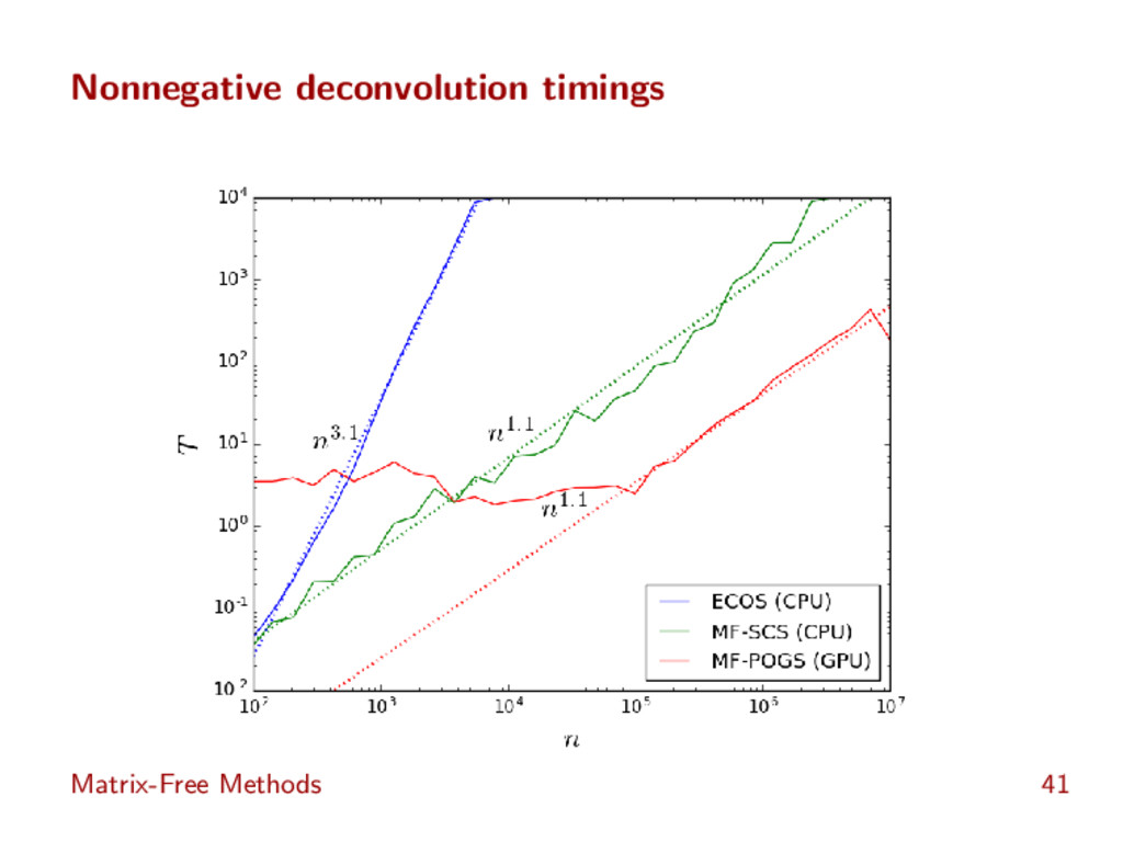
46. Example: Nonnegative deconvolution minimize c ∗ x − b 2 subject to x ≥ 0 variable x ∈ Rn; data c ∈ Rn, b ∈ R2n−1 standard (matrix) method represent c∗ as (2n − 1) × n Toeplitz matrix memory is order n2, solve is order n3 matrix-free method represent c∗ as FAO (implemented via FFT) memory is order n, solve is order n log n Matrix-Free Methods 40
47. Nonnegative deconvolution timings Matrix-Free Methods 41
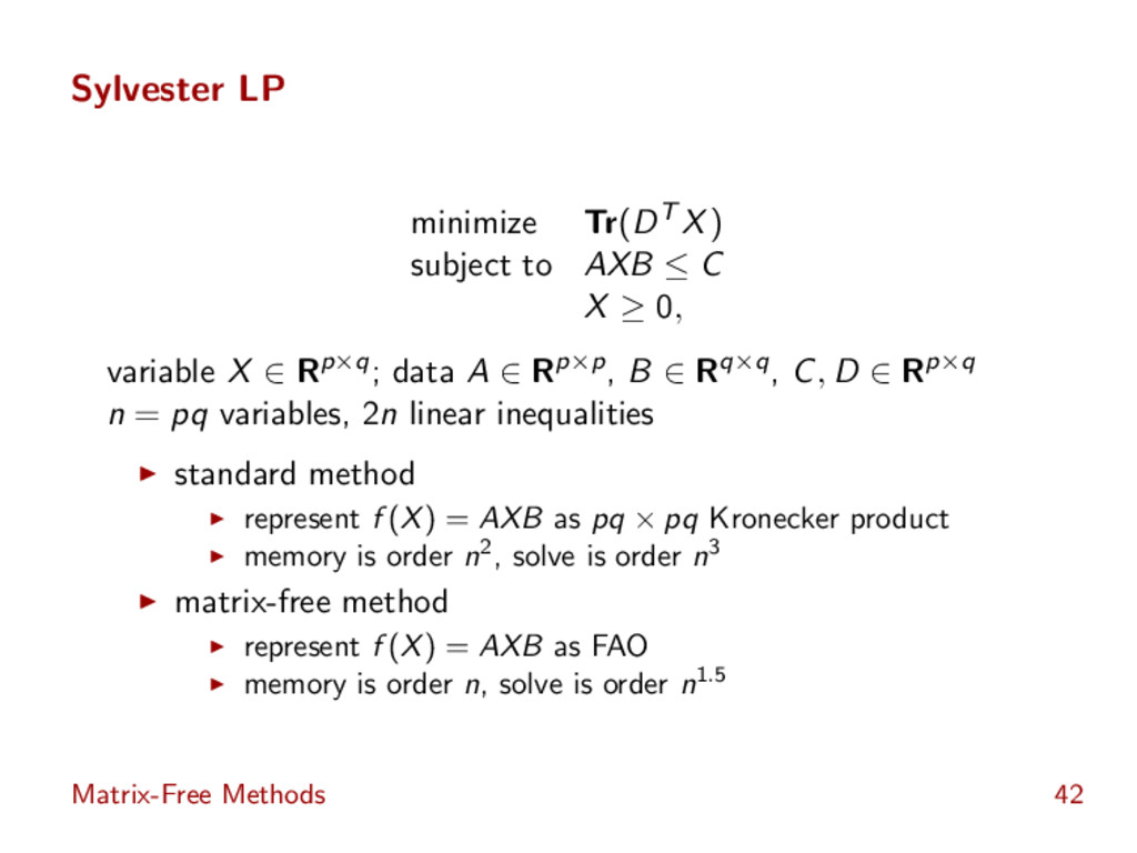
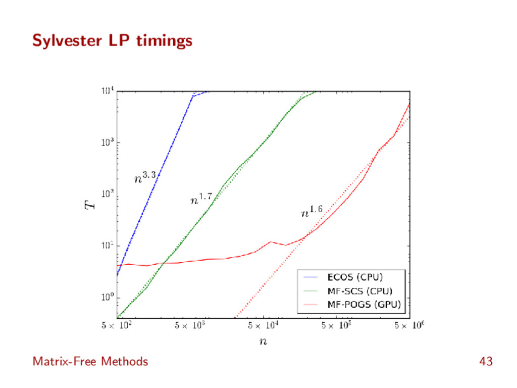
48. Sylvester LP minimize Tr(DT X) subject to AXB ≤ C X ≥ 0, variable X ∈ Rp×q; data A ∈ Rp×p, B ∈ Rq×q, C, D ∈ Rp×q n = pq variables, 2n linear inequalities standard method represent f (X) = AXB as pq × pq Kronecker product memory is order n2, solve is order n3 matrix-free method represent f (X) = AXB as FAO memory is order n, solve is order n1.5 Matrix-Free Methods 42
49. Sylvester LP timings Matrix-Free Methods 43
50. Outline Convex Optimization Examples Matrix-Free Methods Summary Summary 44
51. Summary convex optimization problems arise in many applications small and medium size problems can be solved effectively and conveniently using domain-specific languages, general solvers Summary 45
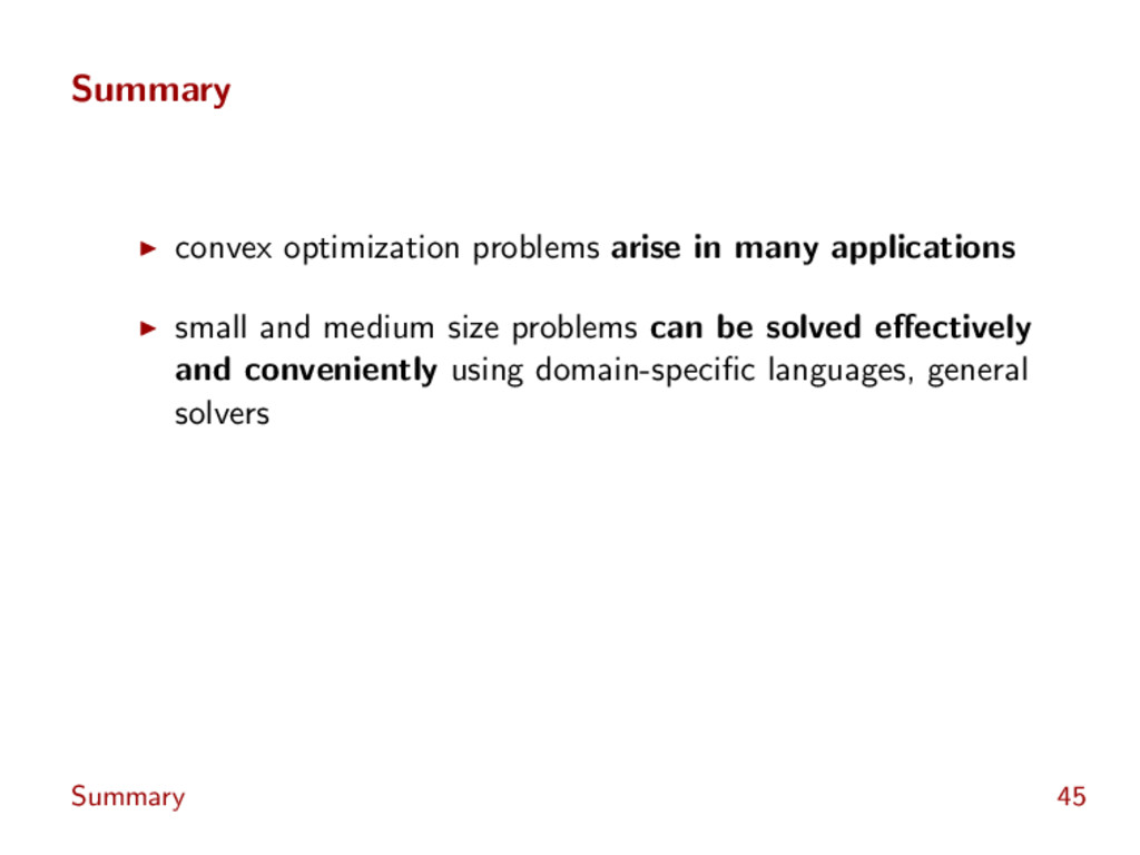
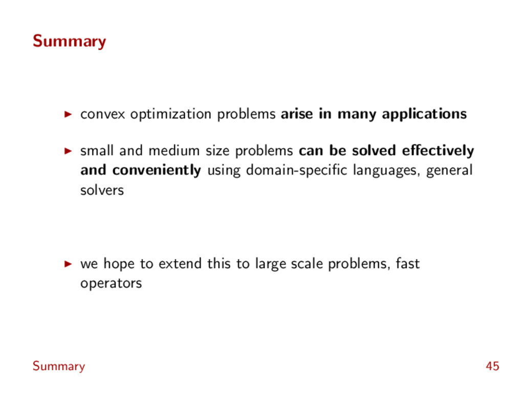
52. Summary convex optimization problems arise in many applications small and medium size problems can be solved effectively and conveniently using domain-specific languages, general solvers we hope to extend this to large scale problems, fast operators Summary 45
53. Resources all available online Convex Optimization (book) EE364a (course slides, videos, code, homework, . . . ) CVX, CVXPY, Convex.jl, SCS, POGS (code) preliminary version of MF-CVXPY (and SCS and POGS): https://github.com/SteveDiamond/cvxpy Summary 46