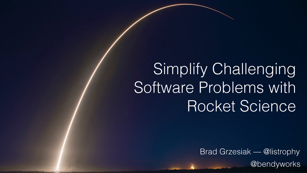
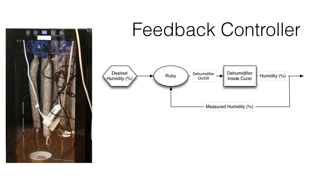
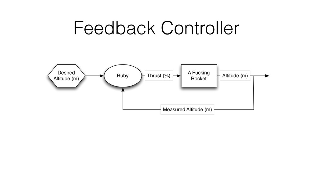
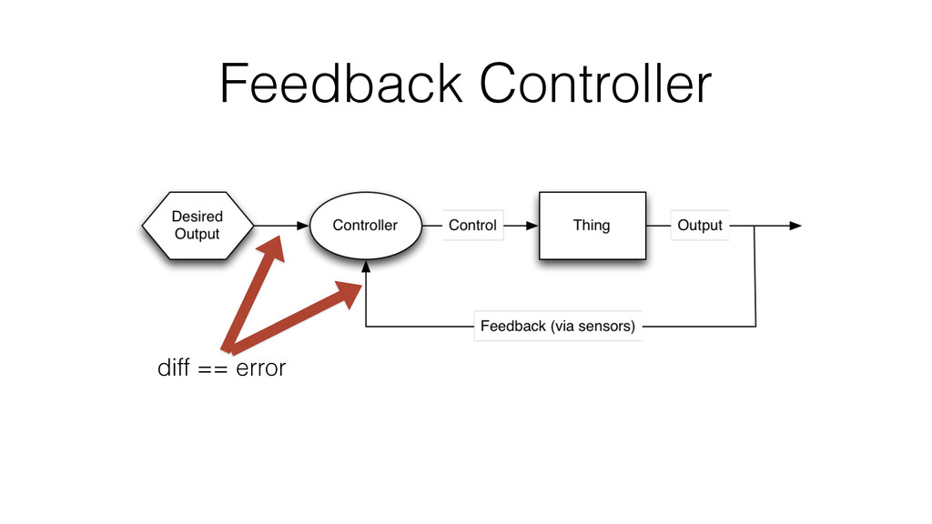
Aerospace engineering is really no more magical than programming, and yet it's shrouded in such mystery and mysticism that practically no one bothers to study it. I'll show you how to apply concepts from rocket science to challenging software problems, allowing you to spend more time coming up with answers rather than interpreting inputs. (40 minute version presented at EuRuKo 2015)
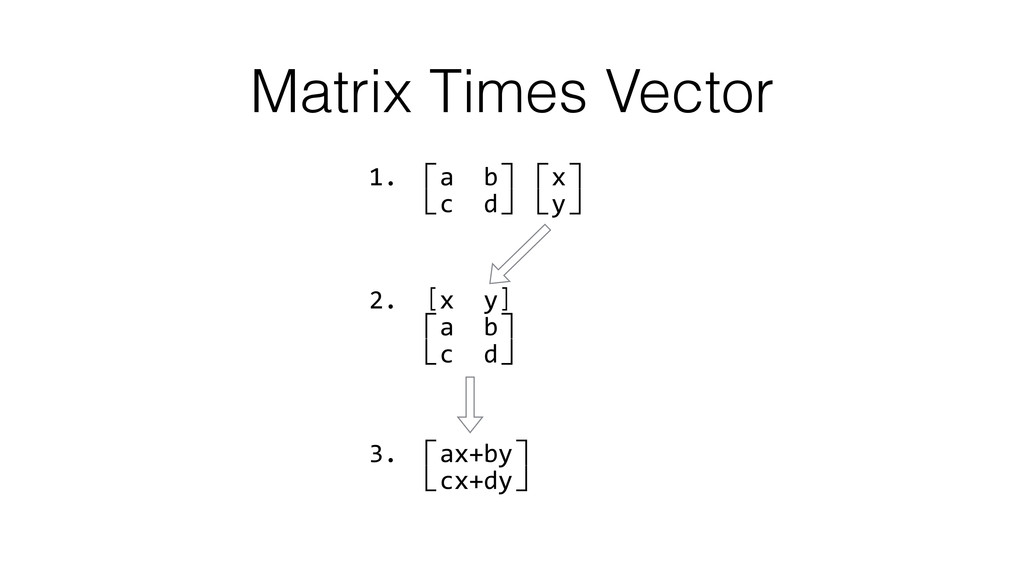
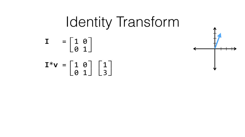
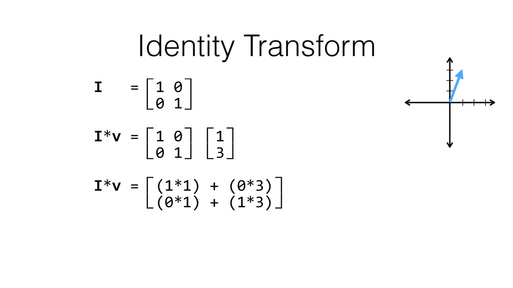
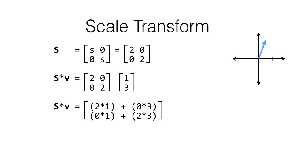
![Matrix Times Vector def matrix_times_vector(m, v) a, b = m[0]](https://files.speakerdeck.com/presentations/7515765ff08748cbbb7c844a1642a810/slide_18.jpg)
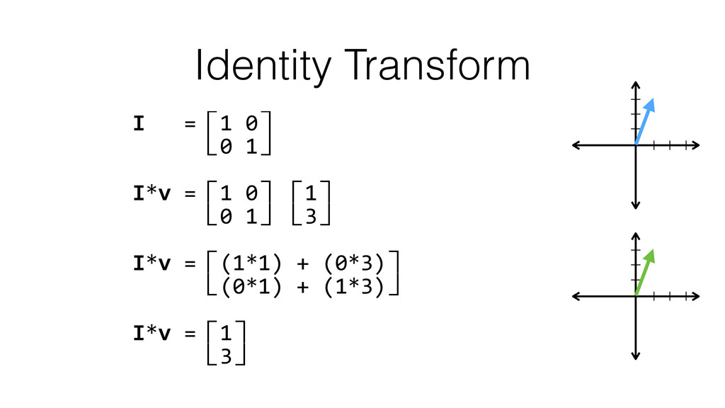
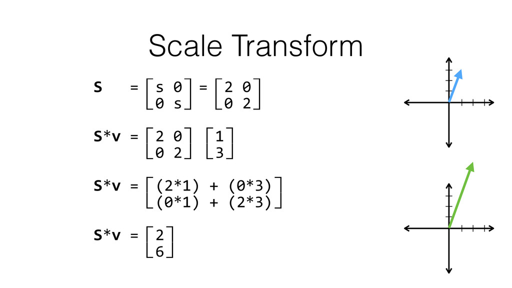
![Matrix Times Vector def matrix_times_vector(m, v) a, b = m[0]](https://files.speakerdeck.com/presentations/7515765ff08748cbbb7c844a1642a810/slide_19.jpg)
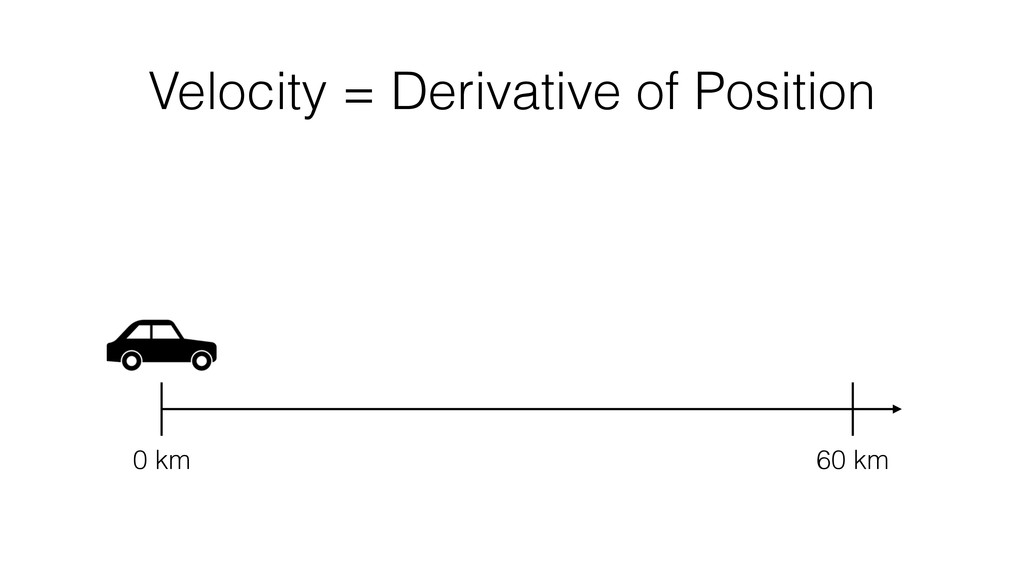
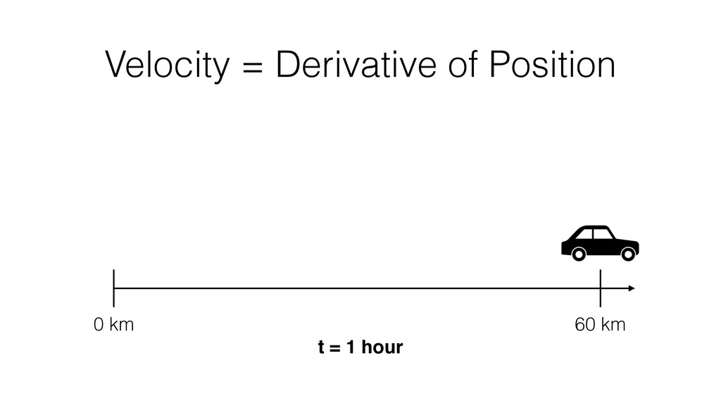
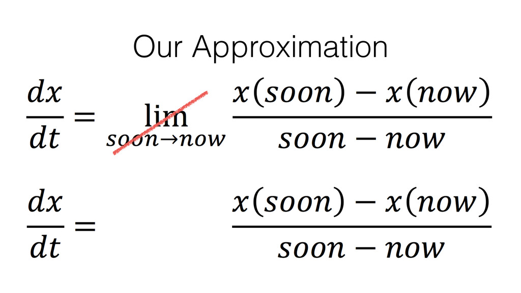
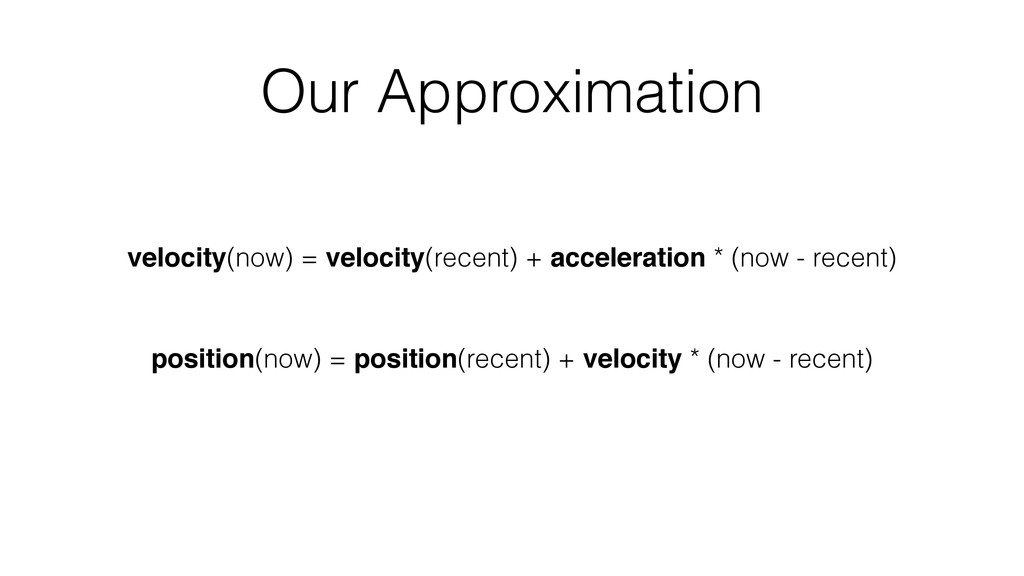
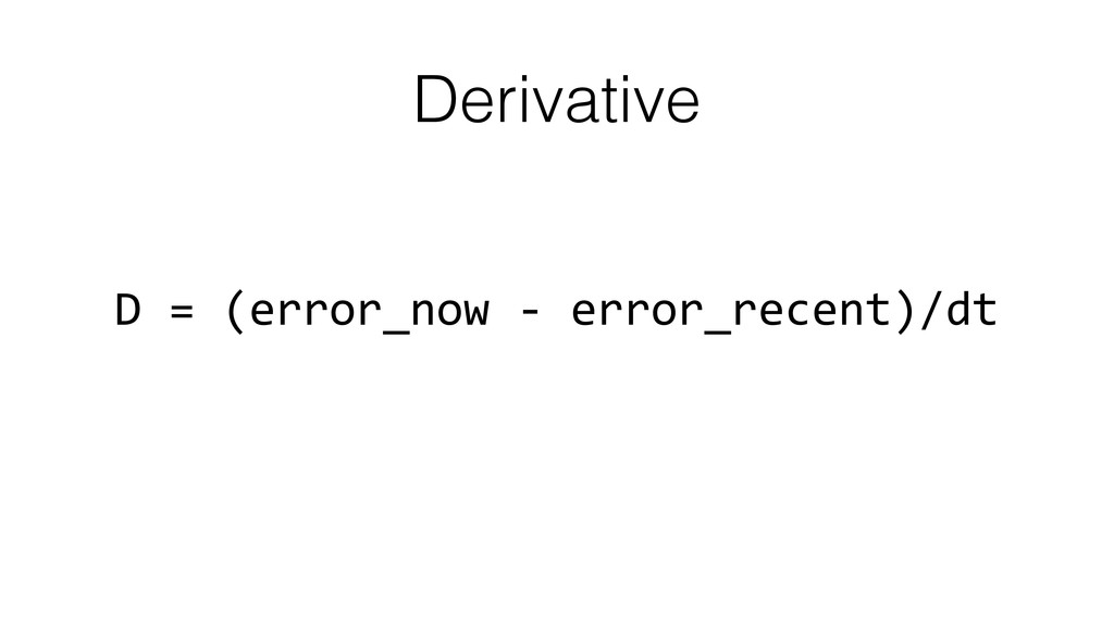
![Our Approximation velocity = [position(now) - position(recent)] / (now -](https://files.speakerdeck.com/presentations/7515765ff08748cbbb7c844a1642a810/slide_86.jpg)
![Our Approximation velocity = [position(now) - position(recent)] / (now -](https://files.speakerdeck.com/presentations/7515765ff08748cbbb7c844a1642a810/slide_87.jpg)
![Our Approximation velocity = [position(now) - position(recent)] / (now -](https://files.speakerdeck.com/presentations/7515765ff08748cbbb7c844a1642a810/slide_88.jpg)
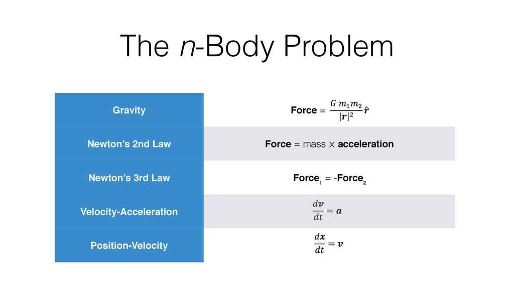
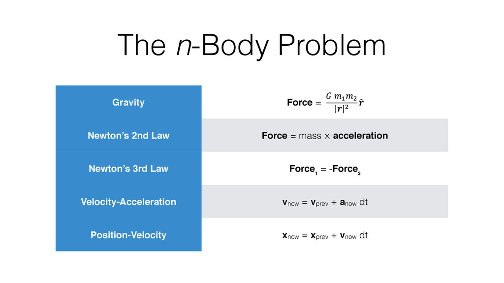
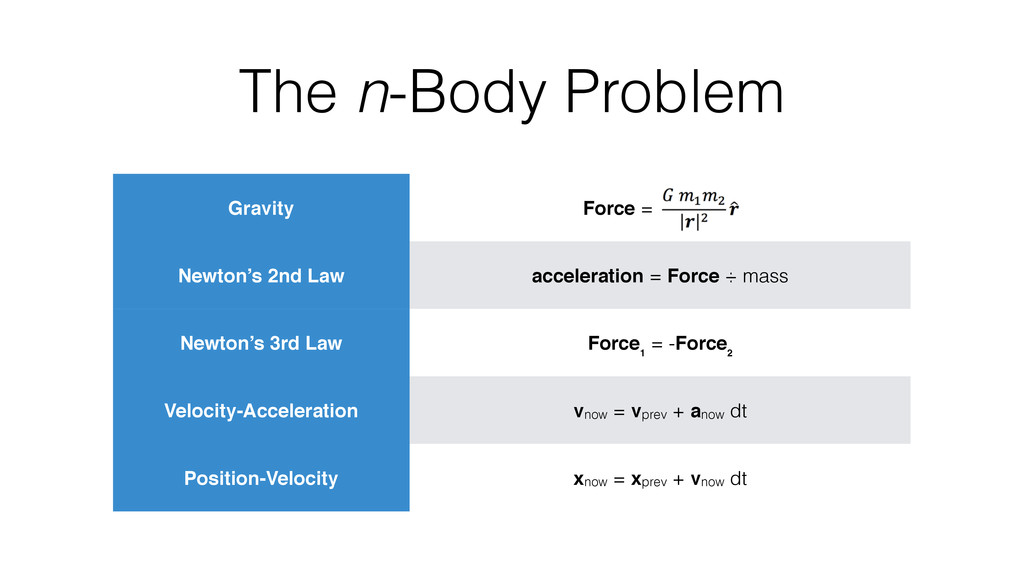
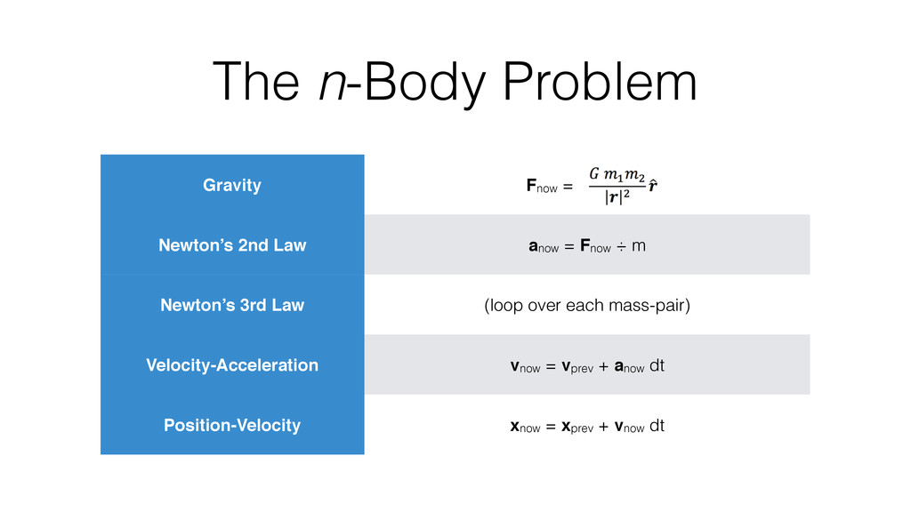
![The n-Body Problem bodies.map do |body| [body, gravity(body, bodies-[body])] end.each](https://files.speakerdeck.com/presentations/7515765ff08748cbbb7c844a1642a810/slide_94.jpg)
![The n-Body Problem def gravity(body, others) others.reduce(Vector[0,0]) do |memo, other|](https://files.speakerdeck.com/presentations/7515765ff08748cbbb7c844a1642a810/slide_95.jpg)
![Thank You! Brad Grzesiak [email protected] @listrophy gitlab.com/listrophy](https://files.speakerdeck.com/presentations/7515765ff08748cbbb7c844a1642a810/slide_118.jpg)