Basics and importing data

How to get any and all data into R. Part of the Zero to R Hero series (http://zerotorhero.wordpress.com).

Transcript

1. www.meetup.com/Montreal-R-User-Group/
2. Basics and loading data Etienne Low-Decarie material in part prepared by Zofia Taranu
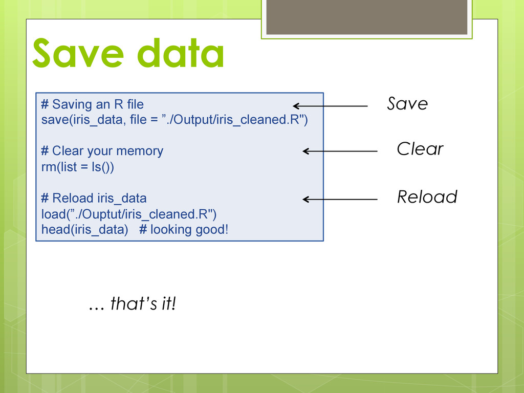
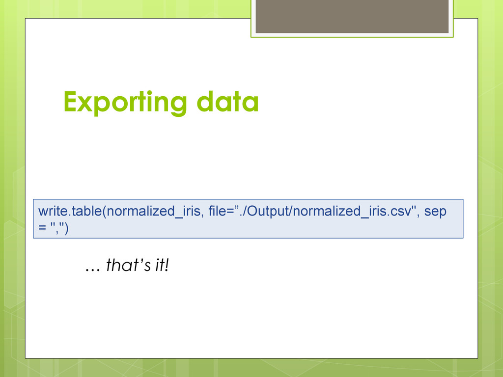
3. Learning Objectives ›  Create an R project ›  Look at Data in R (reminder) ›  Create data that is appropriate for use with R ›  Import data ›  Dealing with broken data files ›  Identifying the problem ›  Fixing it in a spreadsheet ›  Fixing it in R ›  Dealing with bad data formats ›  Reshape from wide to long ›  Save and export data
4. Create an R project ›  Create a basic folder structure for each of your projects ›  Helps you stay organized ›  R will look in here and save to here
5. Create an R project ›  You can download the whole structure with R scripts, data, etc from: ›  https://github.com/zerotorhero/MBSU
6. Create an R project in RStudio ›  In R Studio, create a project in that folder ›  Tells R this is the project and folder your are working on
7. Create an R project ›  In the existing directory you have created or downloaded
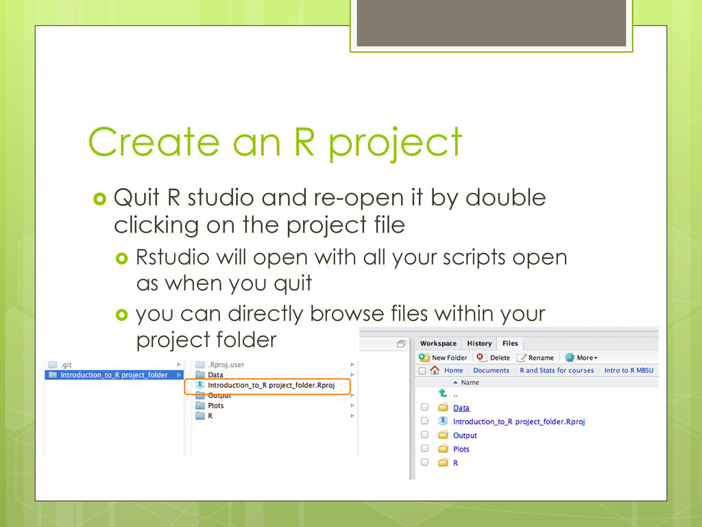
8. Create an R project ›  Quit R studio and re-open it by double clicking on the project file ›  Rstudio will open with all your scripts open as when you quit ›  you can directly browse files within your project folder
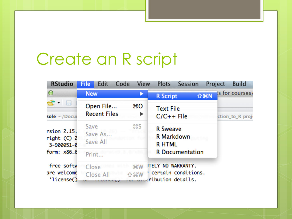
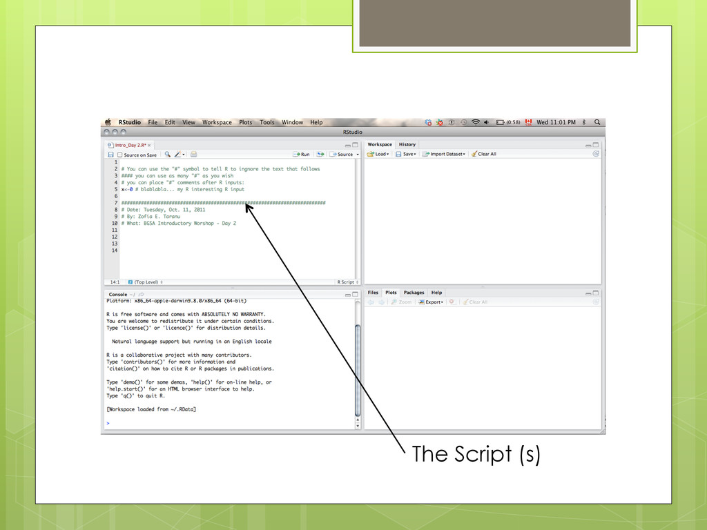
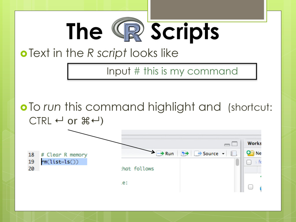
9. The Scripts › What is this? •  A text file that contains all the commands you will use! › Once written and saved, your script file allows you to make changes and re-run analyses with minimal effort!
10. Create an R script
11. The Script (s)
12. Also File-> Open File -> 02_Basics and importing data.R Recommendation create your own new script refer to provided code only if needed avoid copy pasting or running the code directly from script
13. › Text in the R script looks like Input # this is my command › To run this command highlight and (shortcut: CTRL ↵ or ⌘↵) The Scripts
14. Housekeeping ›  Steps you should take before running code ›  Written as a section at the top of scripts
15. Housekeeping › Removes all variables from memory › Prevents errors such as use of older data # Clear R memory rm(list = ls() ) Type this in your R script
16. Commenting ›  # symbol tells R to ignore this ›  commenting/documenting ›  annotate someone’s script is good way to learn ›  remember what you did ›  tell collaborators what you did ›  good step towards reproducible science
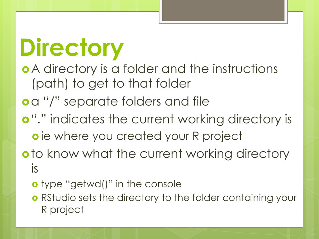
17. Directory › A directory is a folder and the instructions (path) to get to that folder › a “/” separate folders and file › “.” indicates the current working directory is › ie where you created your R project › to know what the current working directory is ›  type “getwd()” in the console ›  RStudio sets the directory to the folder containing your R project
18. Look at data load a built-in data file peek at first few rows structure of the object names of items in the object attributes of the object summary statistics plot of all variable combinations data(CO2) head(CO2) str(CO2) names(CO2) attributes(CO2) summary(CO2) plot(CO2) Working with a data frame
19. Look at data ›  data() ›  head(), str(), names(), attributes(), summary, plot() ›  discuss difference between how you store data and data in R
20. Prep data for R ›  comma separate files (.csv) in Data folder ›  can be created from almost all apps (Excel, LibreOffice, GoogleDocs) ›  file-> save as… .csv
21. Prep data for R ›  short informative column headings ›  starting with a letter ›  no spaces
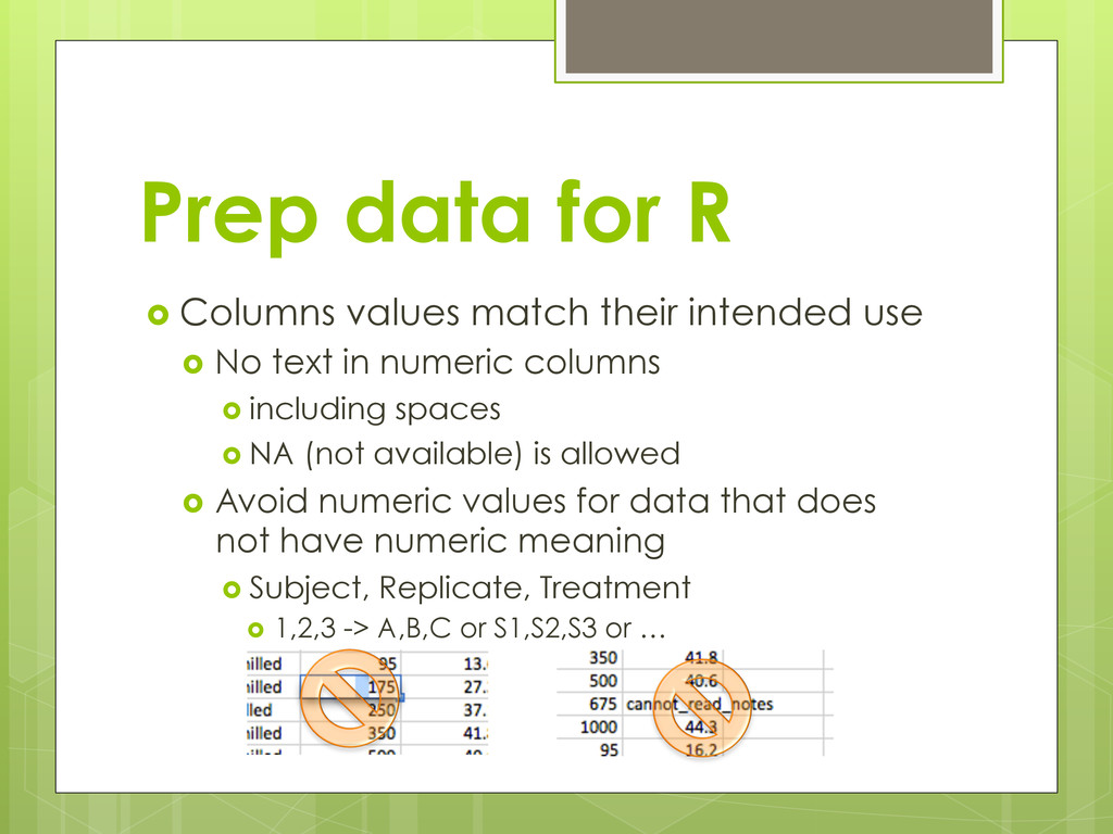
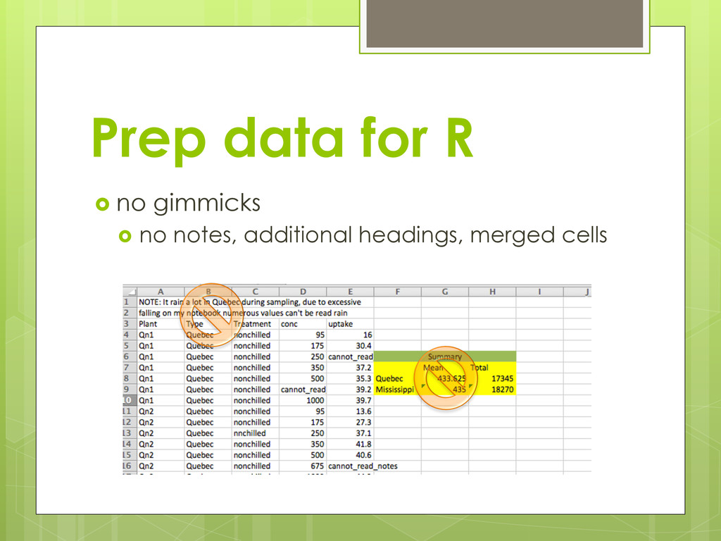
22. Prep data for R ›  Columns values match their intended use ›  No text in numeric columns ›  including spaces ›  NA (not available) is allowed ›  Avoid numeric values for data that does not have numeric meaning ›  Subject, Replicate, Treatment ›  1,2,3 -> A,B,C or S1,S2,S3 or …
23. Prep data for R ›  no gimmicks ›  no notes, additional headings, merged cells
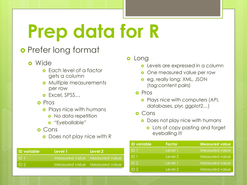
24. Prep data for R ›  Prefer long format ›  Wide ›  Each level of a factor gets a column ›  Multiple measurements per row ›  Excel, SPSS… ›  Pros ›  Plays nice with humans ›  No data repetition ›  “Eyeballable” ›  Cons ›  Does not play nice with R ›  Long ›  Levels are expressed in a column ›  One measured value per row ›  eg. really long: XML, JSON (tag:content pairs) ›  Pros ›  Plays nice with computers (API, databases, plyr, ggplot2…) ›  Cons ›  Does not play nice with humans ›  Lots of copy pasting and forget eyeballing it!
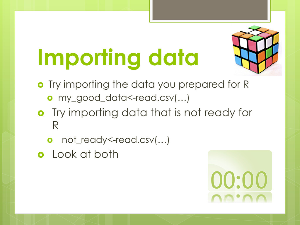
25. Prep data for R ›  Try to prep your data for R or find data you find interesting online and prep it for R ›  Note: it is possible to do all your data prep work within R ›  can be very tedious ›  keeps original data intact ›  can even switch between long and wide
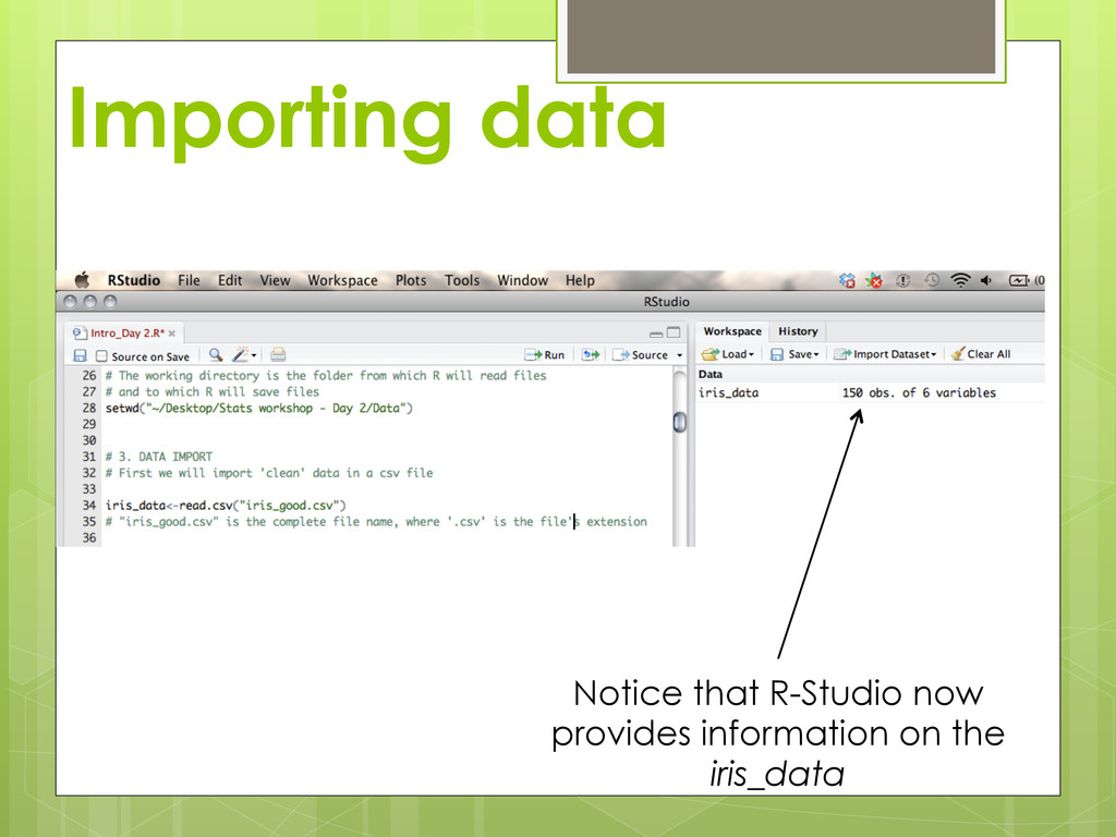
26. Importing data › We will now import the data file iris_data<-­‐read.csv(“./Data/iris_good.csv”)   › Recall: to find out what arguments the command requires, use help “?” ! Object (name) Command (what am I doing) Argument (what am I applying this to) ?read.csv
27. Importing data Notice that R-Studio now provides information on the iris_data
28. Importing data ›  Try importing the data you prepared for R ›  my_good_data<-read.csv(…) ›  Try importing data that is not ready for R ›  not_ready<-read.csv(…) ›  Look at both
29. Manipulate the data ›  Do calculations ›  Eg:
30. Manipulate the data ›  Write your own function ! my.function<-function(arguments){! ! ! ! results<-do.something(arguments)! return(data.frame(results))}! ! area.ellipse<-function(width, length){! ! !area<-pi*(width/2)*(length/2)! ! !return(data.frame(area=area))}! ! with(iris_data, area_ellipse(Sepal.Width, Sepal.Length))! ! ! ! !
31. Manipulate the data ›  Do calculations for each group ›  Eg.: ›  Replace specific values iris_data$mean.sepal.length[iris_data$Species=="setosa"]<-with(iris_data, mean(Sepal.Length)) iris_data$Species[iris_data$Species=="setosa"]<-"Setosa"
32. Manipulate the data ›  Manipulate your data ›  my_data_with_calcs<-my_data ›  means for a group, density, volume…
33. Save data # Saving an R file save(iris_data, file = ”./Output/iris_cleaned.R") # Clear your memory rm(list = ls()) # Reload iris_data load(”./Ouptut/iris_cleaned.R") head(iris_data) # looking good! Save Clear Reload … that’s it!
34. Exporting data write.table(normalized_iris, file=”./Output/normalized_iris.csv", sep = ",") … that’s it!
35. Save and export ›  Manipulate your data ›  save and export : my_data_with_calcs › open it in your previously favourite data app
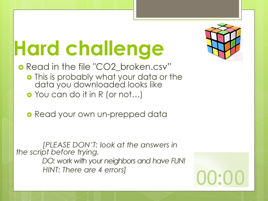
36. Hard challenge ›  Read in the file "CO2_broken.csv” ›  This is probably what your data or the data you downloaded looks like ›  You can do it in R (or not…) ›  Read your own un-prepped data [PLEASE DON’T: look at the answers in the script before trying. DO: work with your neighbors and have FUN! HINT: There are 4 errors]
37. www.meetup.com/Montreal-R-User-Group/
38. Broken data › Try to read in the data file: iris_broken.csv › It didn’t work because the extension was .txt and not .csv iris_data<-read.csv("iris_broken.csv") > iris_data<-read.csv("iris_broken.csv") Error in file(file, "rt") : cannot open the connection In addition: Warning message: In file(file, "rt") : cannot open file 'iris_broken.csv': No such file or directory iris_data<-read.csv("iris_broken.txt") ERROR 1
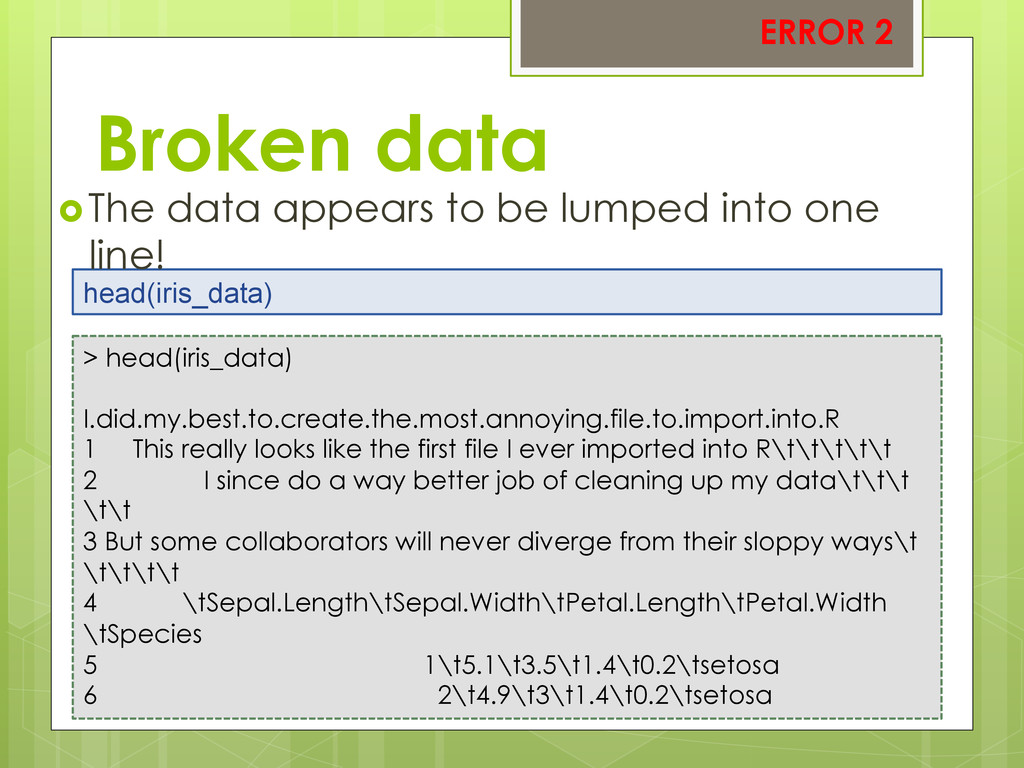
39. Broken data > head(iris_data) I.did.my.best.to.create.the.most.annoying.file.to.import.into.R 1 This really looks like the first file I ever imported into R\t\t\t\t\t 2 I since do a way better job of cleaning up my data\t\t\t \t\t 3 But some collaborators will never diverge from their sloppy ways\t \t\t\t\t 4 \tSepal.Length\tSepal.Width\tPetal.Length\tPetal.Width \tSpecies 5 1\t5.1\t3.5\t1.4\t0.2\tsetosa 6 2\t4.9\t3\t1.4\t0.2\tsetosa head(iris_data) › The data appears to be lumped into one line! ERROR 2
40. Broken data › Re-import the data, but specify the separation among entries •  The sep argument tells R what character separates the values on each line of the file (here; TAB was used) › The first 4 lines are useless › Is anything else strange? iris_data<-read.csv("iris_broken.txt", sep = “”) head(iris_data) str(iris_data) ERROR 2 iris_data<-read.csv("iris_broken.txt", sep = "", skip = 4) head(iris_data) str(iris_data) ERROR 3
41. Broken data › Most continuous variables are listed as factors (categorical) •  Due to missing values entered as “Forgot_this_value” and “na” •  Recall that R only recognizes “NA” (capitalized) > str(iris_data) 'data.frame': 150 obs. of 5 variables: $ Sepal.Length : Factor w/ 35 levels "4.3","4.4","4.5",..: 9 7 5 4 8 12 4 ... $ Sepal.Width : Factor w/ 24 levels "2","2.2","2.3",..: 15 10 12 11 16 ... $ Petal.Length : Factor w/ 45 levels "1","1.1","1.2",..: 5 5 4 6 5 8 5 6 5 ... $ Petal.Width : num 0.2 0.2 0.2 0.2 0.2 0.4 0.3 0.2 0.2 0.1 ... $ Species : Factor w/ 3 levels "setosa","versicolor",..: 1 1 1 1 1 1 ... ERROR 4
42. ERROR 4
43. ERROR 4 read.csv("iris_broken.txt", sep = "", skip = 4, na.strings = c("NA","na","Forgot_this_value")) The fix!
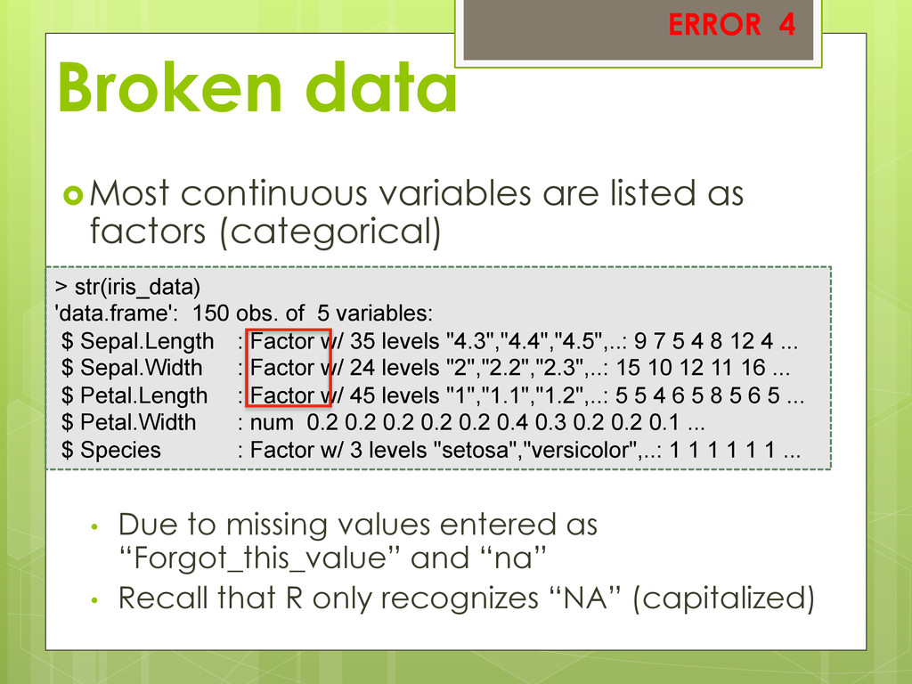
44. Broken data ERROR 5 ›  Ok we’re nearly done! ›  Some variables still appear as factors •  row 23 of Sepal Width was entered as “_3.6” instead of “3.6” ›  Two new arguments we will need •  as.is •  as.numeric Tells R to leave the variable alone Tells R to make the variable numerical iris_data$Sepal.Width[23] class(iris_data$Sepal.Width)
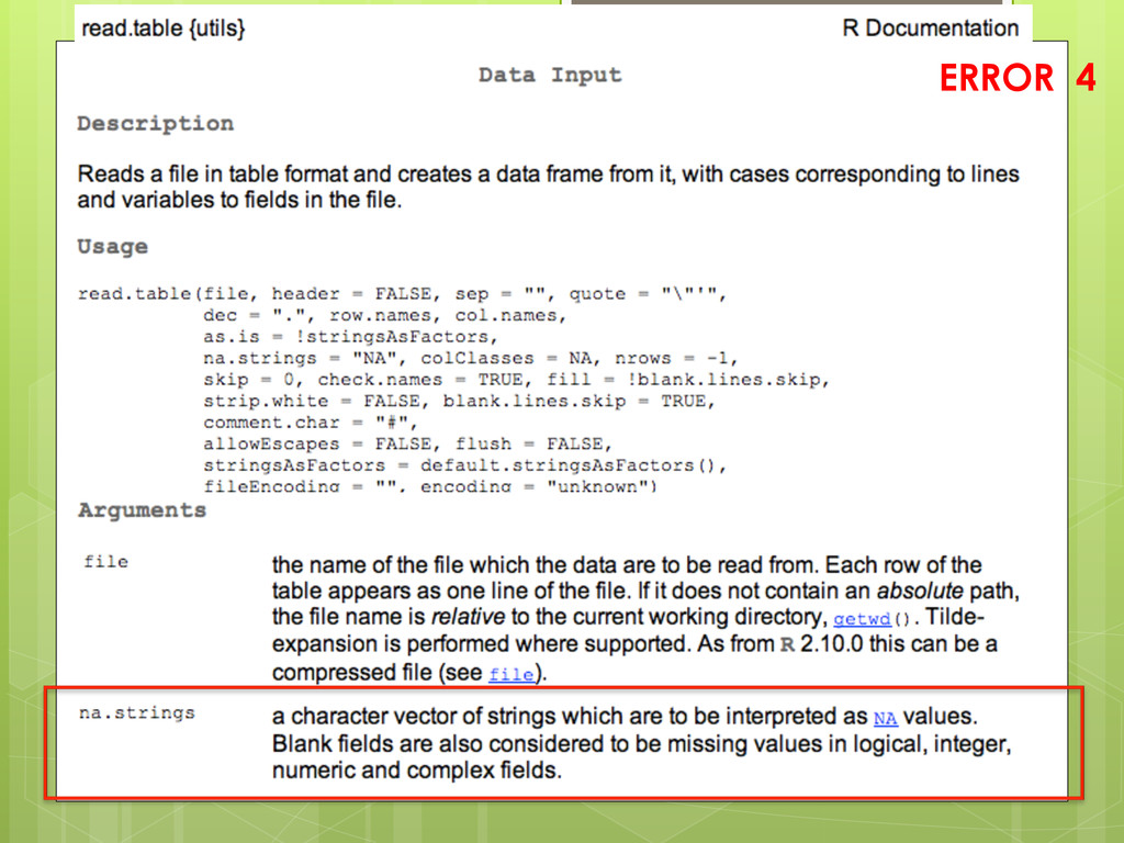
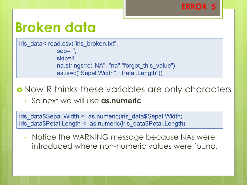
45. Broken data › Now R thinks these variables are only characters •  So next we will use as.numeric •  Notice the WARNING message because NAs were introduced where non-numeric values were found. ERROR 5 iris_data<-read.csv("iris_broken.txt", sep="", skip=4, na.strings=c("NA", "na","forgot_this_value"), as.is=c("Sepal.Width", "Petal.Length")) iris_data$Sepal.Width <- as.numeric(iris_data$Sepal.Width) iris_data$Petal.Length <- as.numeric(iris_data$Petal.Length)
46. www.meetup.com/Montreal-R-User-Group/