Adaptation of microalgae to nutrient fertilization

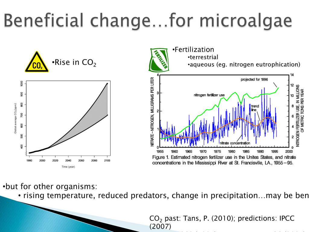
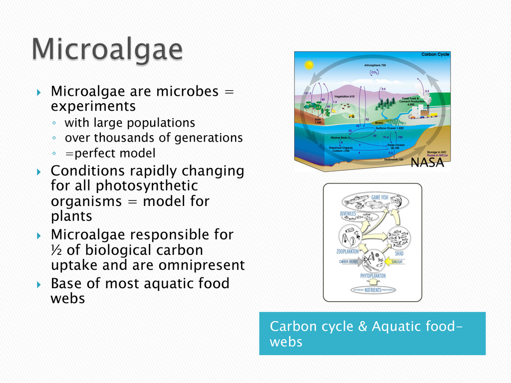
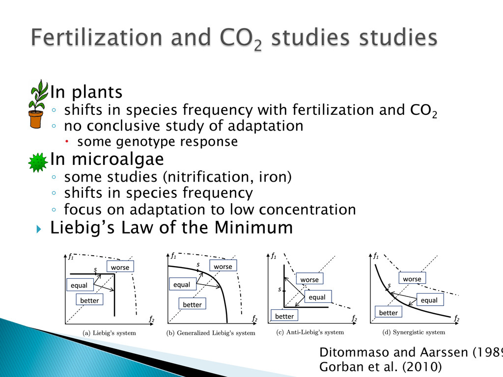
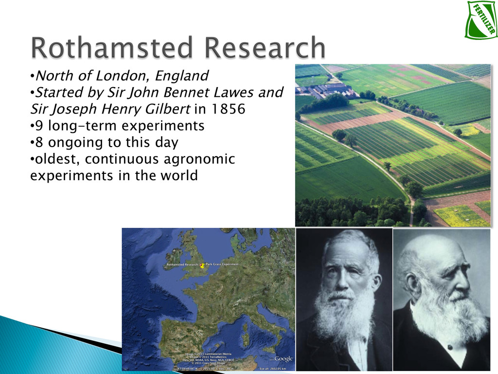
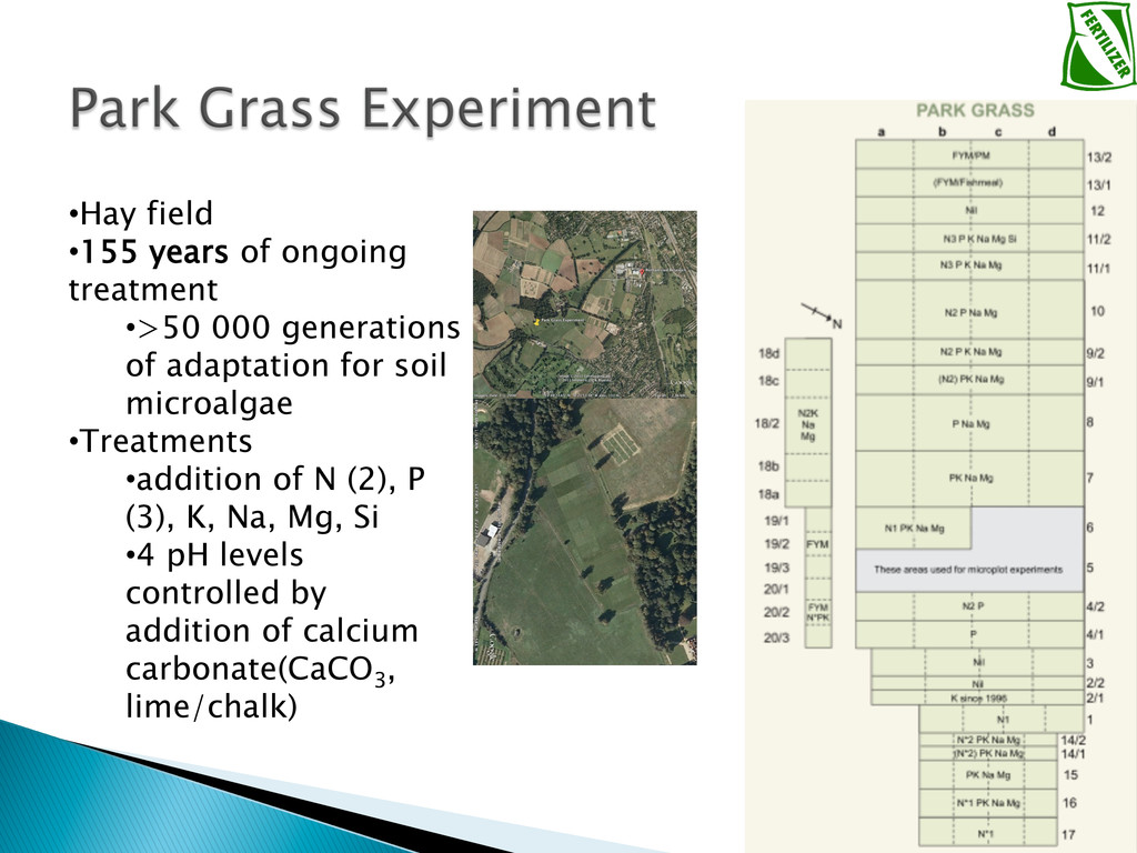
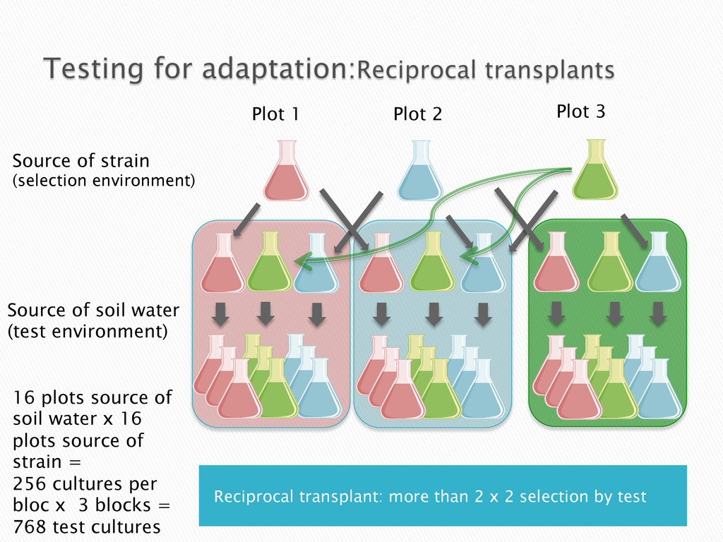
Experimental evolution has predominantly focused on survival and adaptation of organisms subject to stressful changes in their environment. However, in many cases, environmental change shifts conditions towards the optimum of a species. Current theory may not be well suited to predicting the response of organisms to this type of changes. We investigate the adaptation of soil micro-algae to the addition of a variety of fertilizers. We isolated and tested soil micro-algae from plots of the Park Grass Experiment at Rothamsted Research, which have been subject to fertilization treatment continuously for over 150 years. This research will test evolutionary theory in new contexts and will help predict the response of organisms benefiting from global changes, including rising CO2, eutrophication, increased nitrogen availability and rising temperatures.

Transcript

1. Etienne Low-Décarie Graham Bell Gregor Fussmann
2. }  In theory, in experiments and possibly in nature ◦  change is usually for the worst ◦  adaptation seen as a rescue from extinction Bell (2008) Bell and Collins (2008) Chevin et al. 2010 period E, mount pro- n then has deteriora- eles, but at ally benefi- upply rate. fficient to population continually ss depends ts severity produce a n will be l be more expressed vironment mutational ws = w0 –b mutation to depend es, or even ields simi- be able to Evolutionary rescue The outlook is much less benign, however, if lower mean 0.3 0.4 0.5 0.6 0.7 0.8 0.9 –5 –4 –3 –2 –1 0 ln 1/E Mean fitness relative to no change Nu high Nu low Nu very low Figure 2 Effect of environmental change on mean fitness in relation to mutation supply rate. Based on a mutational landscape model as in Fig. 1. From Bell (2008). Bell and Collins
3. CO2 past: Tans, P. (2010); predictions: IPCC (2007) • Rise in CO2 • Fertilization • terrestrial • aqueous (eg. nitrogen eutrophication) • but for other organisms: •  rising temperature, reduced predators, change in precipitation…may be ben
4. Carbon cycle & Aquatic food- webs }  Microalgae are microbes = experiments ◦  with large populations ◦  over thousands of generations ◦  =perfect model }  Conditions rapidly changing for all photosynthetic organisms = model for plants }  Microalgae responsible for ½ of biological carbon uptake and are omnipresent }  Base of most aquatic food webs NASA
5. }  In plants ◦  shifts in species frequency with fertilization and CO2 ◦  no conclusive study of adaptation –  some genotype response }  In microalgae ◦  some studies (nitrification, iron) ◦  shifts in species frequency ◦  focus on adaptation to low concentration }  Liebig’s Law of the Minimum rospects for survival and reproduction. Recently, the Fisher and Haldane are combined (Waxman and Welch 2005): Haldane’s concern is incor- o Fisher’s model by allowing the intensity of selection to vary between ontrivial task to measure the fitness functions and action of selection in now it has been done for many populations and phenotypical traits (King- Pfennig 2007). Special statistical methods for life-history analysis for in- fitness and population growth are developed and tested (Shaw et al. 2008). urther analysis, we do not need exact values of fitness but rather its exis- ome qualitative features. all, let us consider an oversimplified situation with identical organ- n phenotypical treats, fitness W is a function of factor loads: W = fq). This assumption does not take into account physiological adaptation as a protection system and modifies the factor loads. This modification is s of our analysis in the follow-up section, but for now we neglect adapta- onvention about axes direction means that all the partial derivatives of W itive ∂W/∂fi ≤ 0. nition, for a Liebig’s system of factors W is a function of the worst (max- r intensity: W = W(max{f1,...,fq }) (Fig. 2a) and for anti-Liebig’s sys- e function of the best (minimal) factor intensity W = W(min{f1,...,fq }) Such representations as well as the usual formulation of the Law of the require special normalization of factor intensities to compare the loads of ctors. us types of of the system of given state s, the e is given by the f1,f2) = W(s). rates the area with (“better rom the line with (“worse In Liebig’s (a) and iebig’s systems (b) tter conditions is nti-Liebig’s” nd the general stems (d) the area Ditommaso and Aarssen (1989 Gorban et al. (2010) tence and some qualitative features. First of all, let us consider an oversimplified situation with identical organ- isms. Given phenotypical treats, fitness W is a function of factor loads: W = W(f1,...,fq). This assumption does not take into account physiological adaptation that works as a protection system and modifies the factor loads. This modification is in the focus of our analysis in the follow-up section, but for now we neglect adapta- tion. The convention about axes direction means that all the partial derivatives of W are nonpositive ∂W/∂fi ≤ 0. By definition, for a Liebig’s system of factors W is a function of the worst (max- imal) factor intensity: W = W(max{f1,...,fq }) (Fig. 2a) and for anti-Liebig’s sys- tem it is the function of the best (minimal) factor intensity W = W(min{f1,...,fq }) (Fig. 2c). Such representations as well as the usual formulation of the Law of the Minimum require special normalization of factor intensities to compare the loads of different factors. Fig. 2 Various types of organization of the system of factors. For a given state s, the bold solid line is given by the equation W(f1,f2) = W(s). This line separates the area with higher fitness (“better conditions”) from the line with lower fitness (“worse conditions”). In Liebig’s (a) and generalized Liebig’s systems (b) the area of better conditions is convex, in “anti-Liebig’s” systems (c) and the general synergistic systems (d) the area of worse conditions is convex. The dot dash line shows the border of survival. On the dashed line, the factors are equally important (f1 = f2)
6. • North of London, England • Started by Sir John Bennet Lawes and Sir Joseph Henry Gilbert in 1856 • 9 long-term experiments • 8 ongoing to this day • oldest, continuous agronomic experiments in the world
7. • Hay field • 155 years of ongoing treatment • >50 000 generations of adaptation for soil microalgae • Treatments • addition of N (2), P (3), K, Na, Mg, Si • 4 pH levels controlled by addition of calcium carbonate(CaCO3 , lime/chalk)
8. The team, sampling Experiments •  Soil water isolated from 16 plots •  Lab strain of Chlamydomonas bio- assay of soil water •  Micro-algae isolated from 16 plots •  3 block replication of complete factorial reciprocal transplant Gregor Graham
9. Reciprocal transplant: more than 2 x 2 selection by test Source of strain (selection environment) Plot 1 Plot 2 Plot 3 Source of soil water (test environment) 16 plots source of soil water x 16 plots source of strain = 256 cultures per bloc x 3 blocks = 768 test cultures
10. Accumulation of conditionaly deleterious mutations Source of strain Source of test environment 1 2 3 1 2 3 Cell density 0.0 0.5 1.0 1.5 2.0 2.5 3.0 Specific adaptation with tradeoff or combination of adaptation and conditionaly deliterious mutations Source of strain Source of test environment 1 2 3 1 2 3 Cell density 1 2 3 4 5 Specific adaptation Source of strain Source of test environment 1 2 3 1 2 3 Cell density 1 2 3 4 5 Conditional deleterious mut. Tradeoff Specific adaptation No difference between strains Source of strain Source of test environment 1 2 3 1 2 3 Cell density 1.0 1.5 2.0 2.5 3.0 Non specific adapatation Source of strain Source of test environment 1 2 3 1 2 3 Cell density 1 2 3 4 5 fertilization - + fertilization - + No evolution Non-specific adaptation
11. • Davies and Snaydon (1973-1982) • single generation transplants • differences small and possibly not evolutionary/genetic • single species ° fertilized with P • no fertilization responded significantly to Ca up to 54 mg 1-' Ca (F from unlimed plots did not respond significantly t response to Ca between population types (lim 'population types x Ca' interaction, was significa the error mean square or the 'populations with test is more stringent, since it measures differen relative to differences between populations withi a~~ 4-5 (a) 015 3 E " 40 30 C a 5 SD "' ~LSD0 010 I (P =0-05) S a - 0~~~~1, .2 011 ,/oz *//a 005 -C ~~ ~~~~ 2-5- 1) 0 0 2 6 18 54 162 t Calcium concentration (mg 1-') in culture soln FIG. 1. The effect of Ca concentration in sand cultu yield per plant of Anthoxanthum odoratum popu Experiment. (a) The effect of Ca concentration (3-19 (a) and unlimed (0) plots. Each point is the mean ship between the Ca response of each population efficient of loge dry weight yield on loge Ca concen and the soil pH of its s Over the range 2-54 mg I- ' Ca, the response significantly from linearity, when loge dry weig concentration (Fig. la). It is therefore possible to lation, over that range, as the linear regressi population to Ca, as measured by the regressio 0 90, P<0.01) with the soil pH of the source p regression coefficient of the most responsive pop of the least responsive population. There are no av of soils from the Park Grass plots (A. E. Johnst ° fertilized with Ca • no fertilization
12. Clamydomonas in soil water from each plot Transformed yield (sqrt of cell/uL) 0 10 20 30 40 50 • • • • • • • • • • • 12 17 1 3 4/2 15 10 2/24/1 1611/1 7 14/2 8 9/211/2 Plot ID Nutrient Ammonium Sulphate Magnesium Sulphate Potassium Sulphate Sodium Nitrate Sodium Silicate Sodium Sulphate Triple Superphosphate 12 17 1 3 4/2 15 10 2/24/1 1611/1 7 14/2 8 9/211/2 Nutrient level 0 1 2 3
13. Growth of collected strains in reciprocal transplant Plot origin of algal strain Plot origin of soil water Plot 12 Plot 2−2 Plot 3 Plot 1 Plot 17 Plot 4−1 Plot 4−2 Plot 8 Plot 15 Plot 7 Plot 10 Plot 16 Plot 14−2 Plot 9−2 Plot 11−1 Plot 11−2 Replicate: 1 Plot 12 Plot 2−2 Plot 3 Plot 1 Plot 17 Plot 4−1 Plot 4−2 Plot 8 Plot 15 Plot 7 Plot 10 Plot 16 Plot 14−2 Plot 9−2 Plot 11−1 Plot 11−2 Replicate: 2 Plot 12 Plot 2−2 Plot 3 Plot 1 Plot 17 Plot 4−1 Plot 4−2 Plot 8 Plot 15 Plot 7 Plot 10 Plot 16 Plot 14−2 Plot 9−2 Plot 11−1 Plot 11−2 Replicate: 3 Plot 12 Plot 2−2 Plot 3 Plot 1 Plot 17 Plot 4−1 Plot 4−2 Plot 8 Plot 15 Plot 7 Plot 10 Plot 16 Plot 14−2 Plot 9−2 Plot 11−1 Plot 11−2 Cell densit standardiz of strain a 0.5 1.0 1.5 Growth of collected strains in reciprocal transplant 2 3 Cell density standardized by origin of strain and of soil water 0.5 1.0 1.5 fertilization - + fertilization - +
14. Triple Superphosphate Magnesium Sulphate Triple Superphosphate Nutrient level in plot origin of algal strain Nutrient level in plot origin of soil water 0 1 Replicate: 1 0 1 Replicate: 2 0 1 Replicate: 3 0 1 Log cell density 1 2 3 4 Magnesium Sulphate Nutrient level in plot origin of algal strain Nutrient level in plot origin of soil water 0 1 Replicate: 1 0 1 Replicate: 2 0 1 Replicate: 3 0 1 Log cell density 1 2 3 4
15. Correlation between Chlamydomonas density and strain density Mean log cell density in Chlamydomonas bio−assay (one value per plot source of assay soil water) Log cell density in reciprocal transplant 1 2 3 4 Replicate: 1 • • • • • • • • • • • • • • • • • • • • • • • • • • • • • • • • • • • • • • • • • • • • • • • • • • • • • • • • • • • • • • • • • • • • • • • • • • • • • • • • • • • • • • • • • • • • • • • • • • • • • • • • • • • • • • • • • • • • • • • • • • • • • • • • • • • • • • • • • • • • • • • • • • • • • • • • • • • • • • • • • • • • • • • • • • • • • • • • • • • • • • • • • • • • • • • • • • • • • • • • • • • • • • • • • • • • • • • • • • • • • • • • • • • • • • • • • • • • • • • • • • • • • 2.3 2.4 2.5 2.6 2.7 2.8 2.9 Replicate: 2 • • • • • • • • • • • • • • • • • • • • • • • • • • • • • • • • • • • • • • • • • • • • • • • • • • • • • • • • • • • • • • • • • • • • • • • • • • • • • • • • • • • • • • • • • • • • • • • • • • • • • • • • • • • • • • • • • • • • • • • • • • • • • • • • • • • • • • • • • • • • • • • • • • • • • • • • • • • • • • • • • • • • • • • • • • • • • • • • • • • • • • • • • • • • • • • • • • • • • • • • • • • • • • • • • • • • • • • • • • • • • • • • • • • • • • • • • • • • • • • • • • • • • • • • • • • • • • • • 2.3 2.4 2.5 2.6 2.7 2.8 2.9 Replicate: 3 • • • • • • • • • • • • • • • • • • • • • • • • • • • • • • • • • • • • • • • • • • • • • • • • • • • • • • • • • • • • • • • • • • • • • • • • • • • • • • • • • • • • • • • • • • • • • • • • • • • • • • • • • • • • • • • • • • • • • • • • • • • • • • • • • • • • • • • • • • • • • • • • • • • • • • • • • • • • • • • • • • • • • • • • • • • • • • • • • • • • • • • • • • • • • • • • • • • • • • • • • • • • • • • • • • • • • • • • • • • • • • • • • • • • • • • • • • • • • • • • • • • • • • • • • • • • • 2.3 2.4 2.5 2.6 2.7 2.8 2.9 Strain.plot • Plot 1 • Plot 10 • Plot 11−1 • Plot 11−2 • Plot 12 • Plot 14−2 • Plot 15 • Plot 16 • Plot 17 • Plot 2−2 • Plot 3 • Plot 4−1 • Plot 4−2 • Plot 7 • Plot 8 • Plot 9−2
16. }  Weak evidence for specific adaptation }  Accumulation of conditionally deleterious mutations }  No evidence for specific adaptation ◦  No evidence of consistent physiological growth response ◦  Difficulty in detecting evolution other than specific local adaptation with tradeoff in larger than 2x2 selection by test environment matrices Specific adaptation to high CO2 unlikely?
17. }  Predicting ◦  atmospheric CO2 ◦  ecological change/species shifts ◦  crop yield ◦  algal blooms }  Optimizing algal bio fuel production }  effect on lab strains of benign environment }  …
18. }  Past and present members of the Bell and Fussmann Labs: ◦  Kathy Tallon, Mark Jewell, Tyler Moulton, Adam Gregory Meyer… }  Yves Prairie, Neil Price, Michel Loreau, Irene Gregory-Eaves, Mark Romer and countless others http://etienne.webhop.org etienne.low-decarie@mail.mcgill.ca Lorne Trottier Philip Carpenter Mr. Ian Clark Dr. Penny Hirsch Dr. Jonathan Storkey,