Hadley Ecosystem: Reshape, Plyr, GGplot

Presented at: http://www.meetup.com/Montreal-R-User-Group/events/88570532/

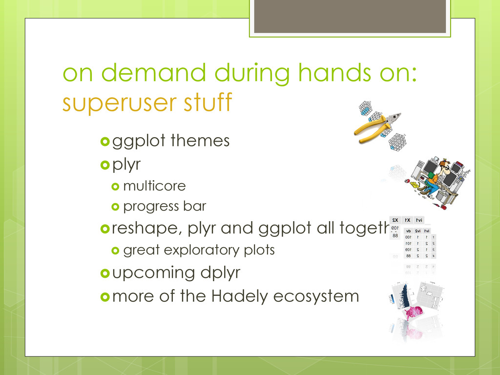
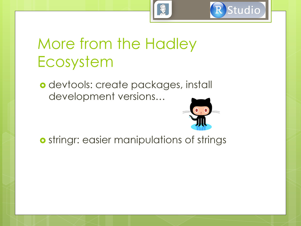
We will give you a fly over of a few of the packages Hadley Wickham and his collaborators have created. Many of us now use these packages in every project we tackle and they have become an essential tool of the R enthusiast tool box. A brief tutorial providing the key features and how to implement them will be presented for each package, each followed by a hands on application exercise. Tips and trick for super users will also be provided.

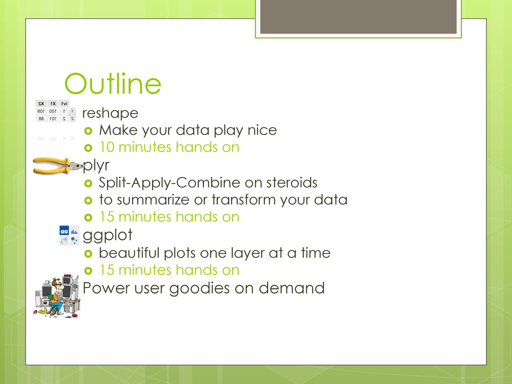
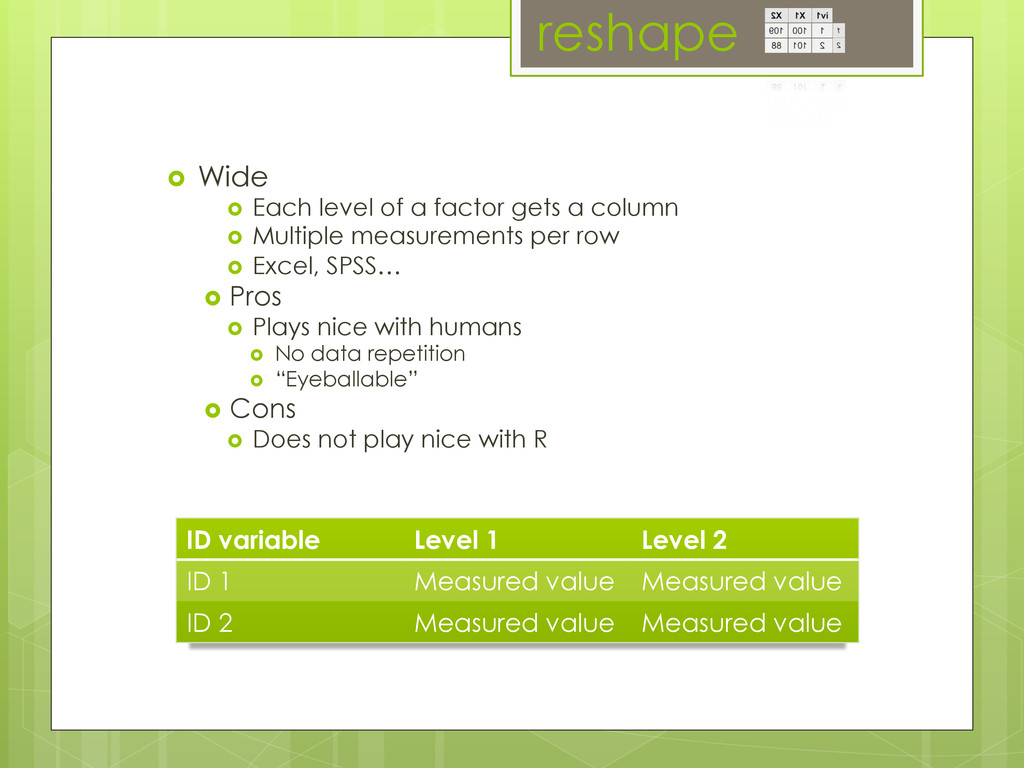
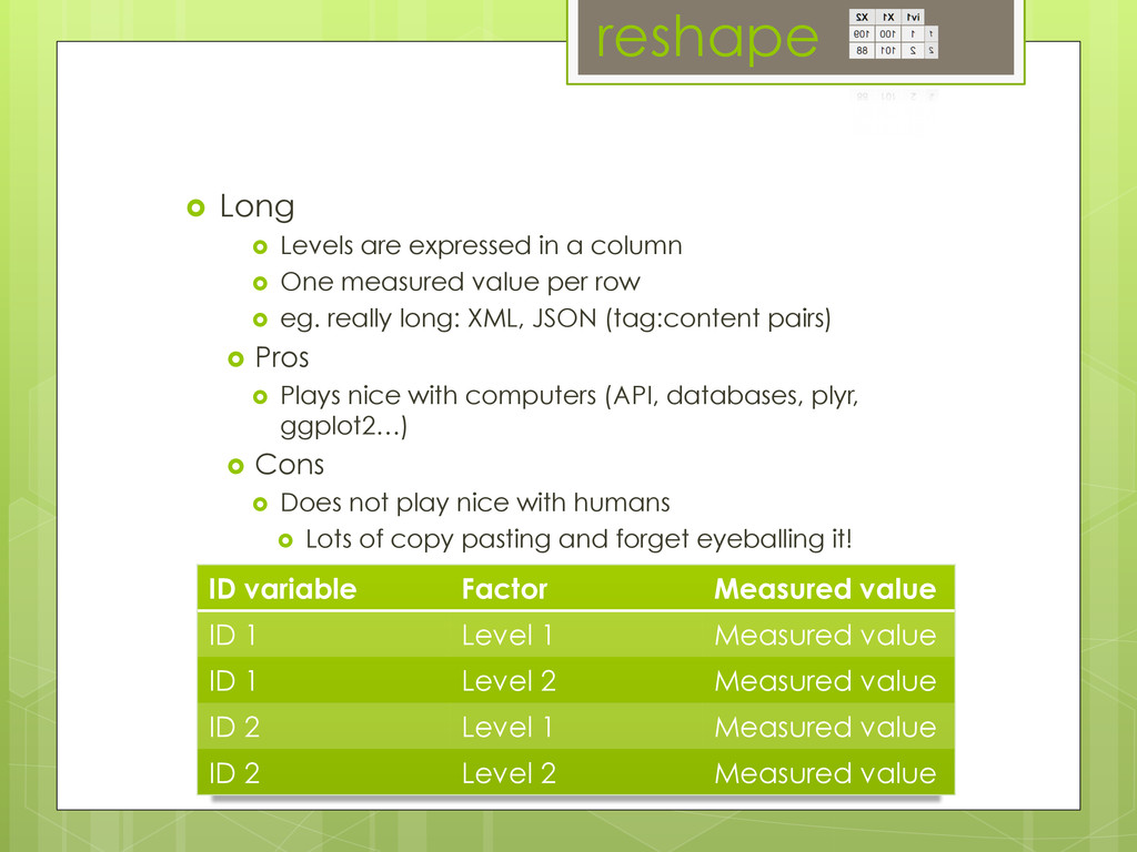
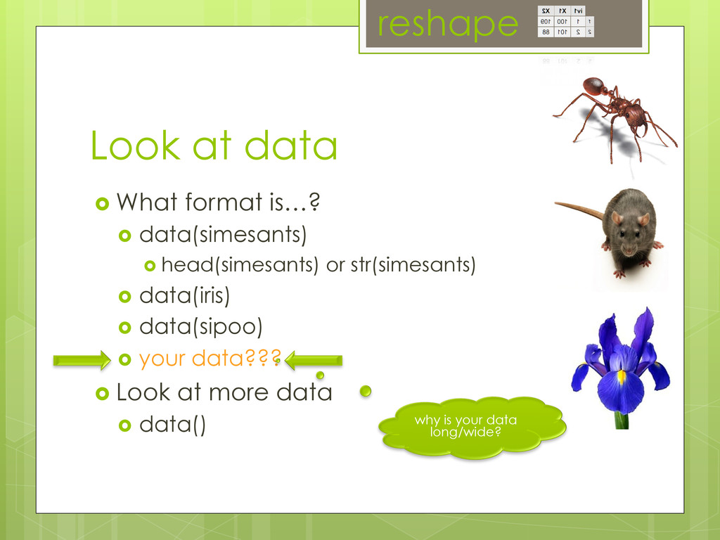
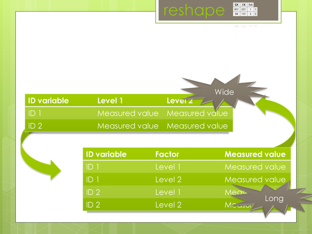
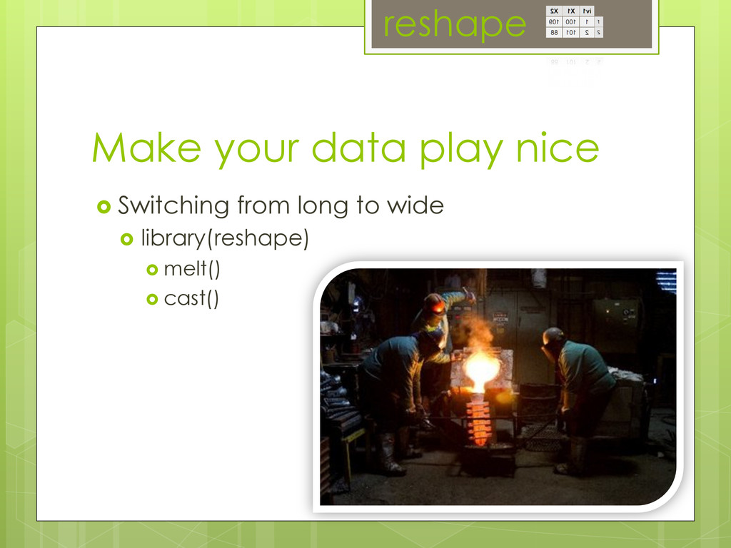
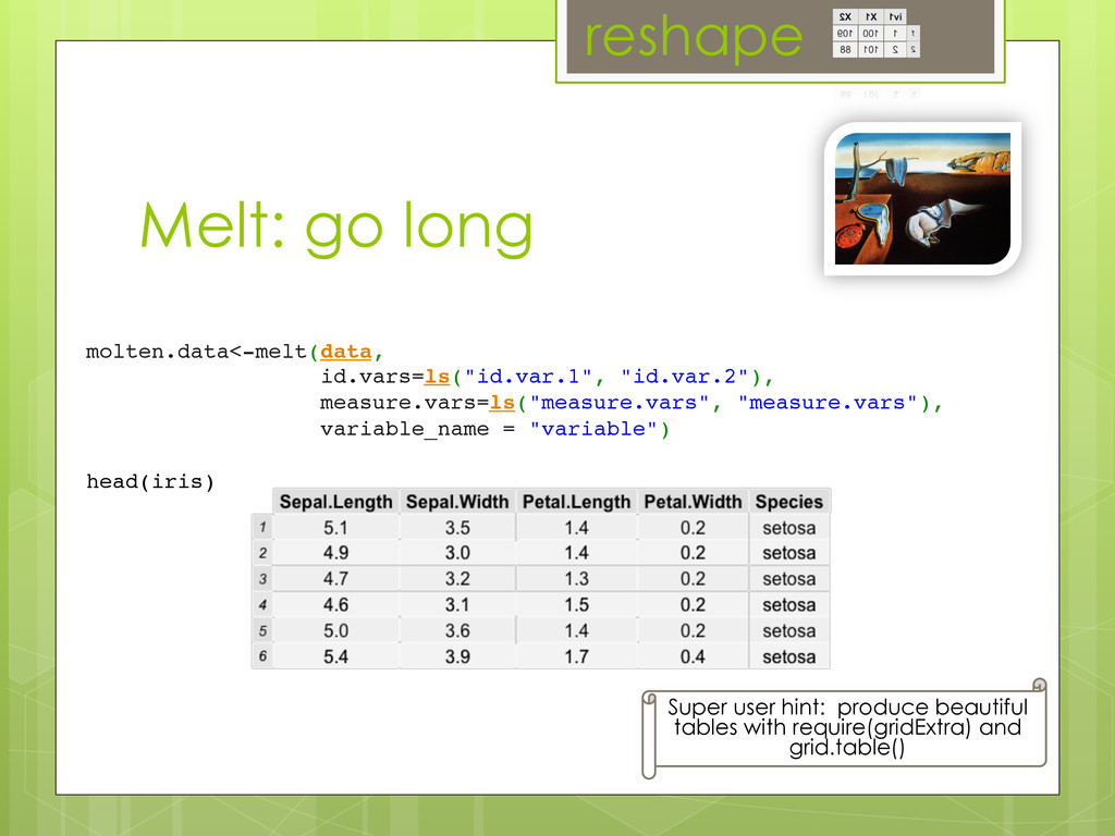
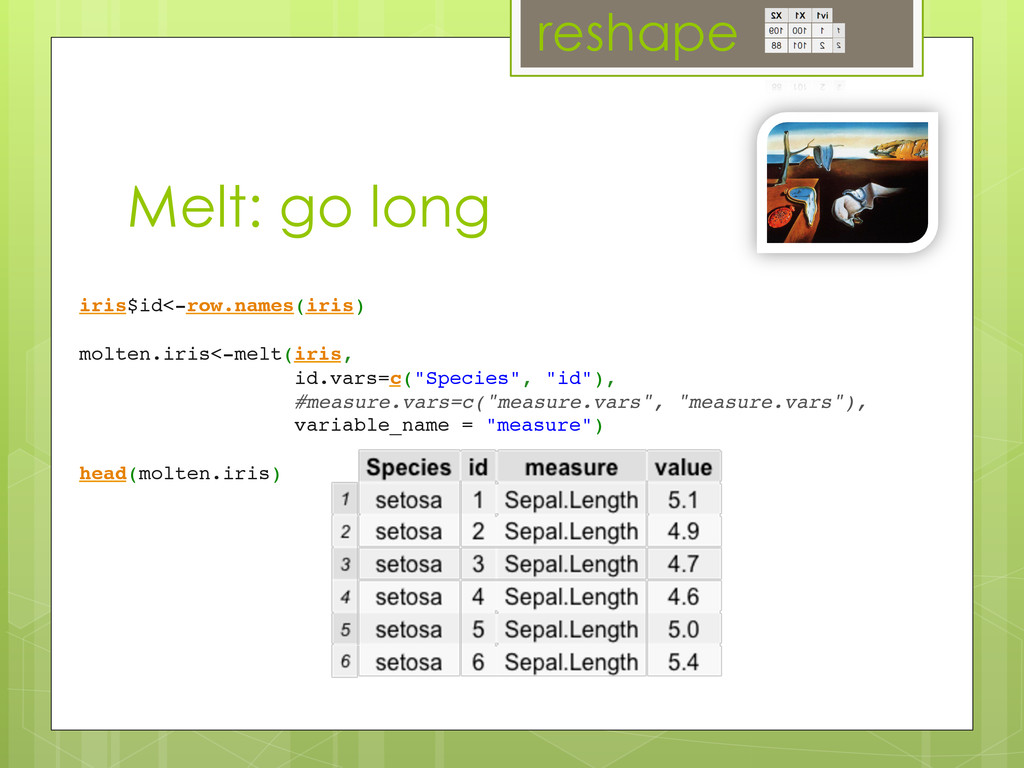
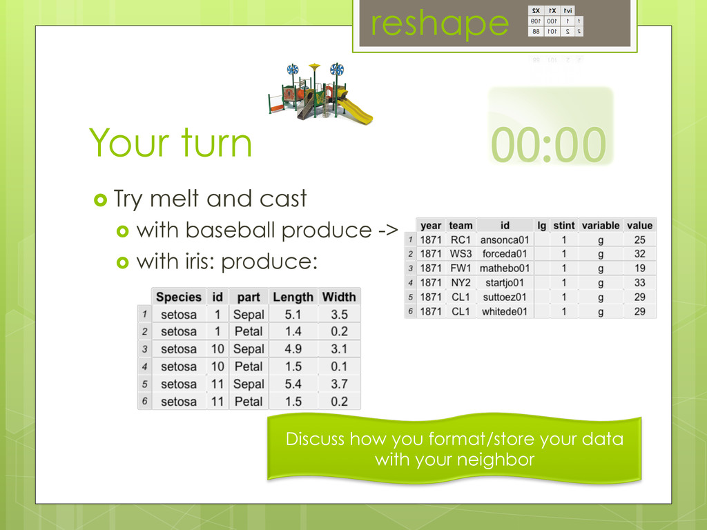
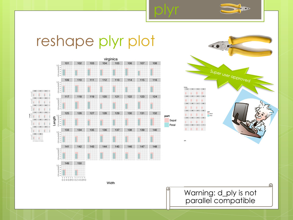
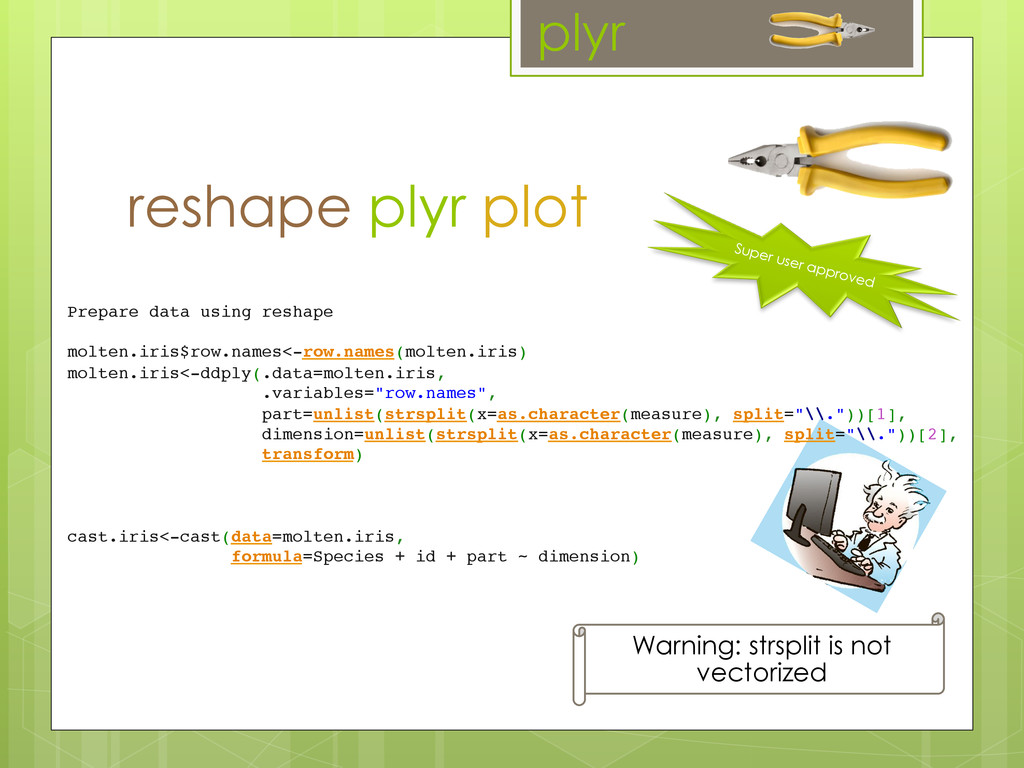
-reshape: make your data play nice (Too many columns, no problem)

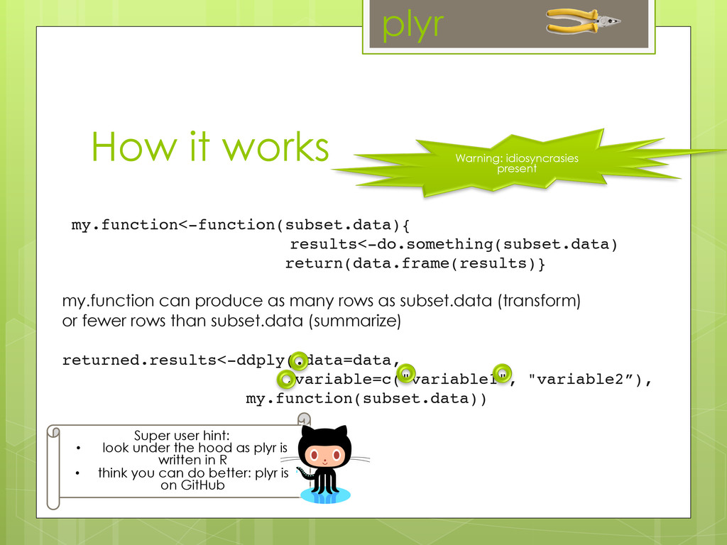
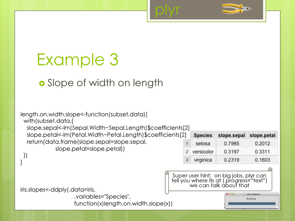
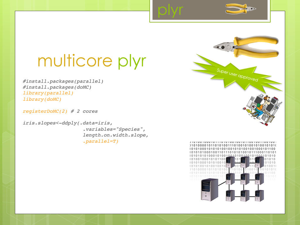
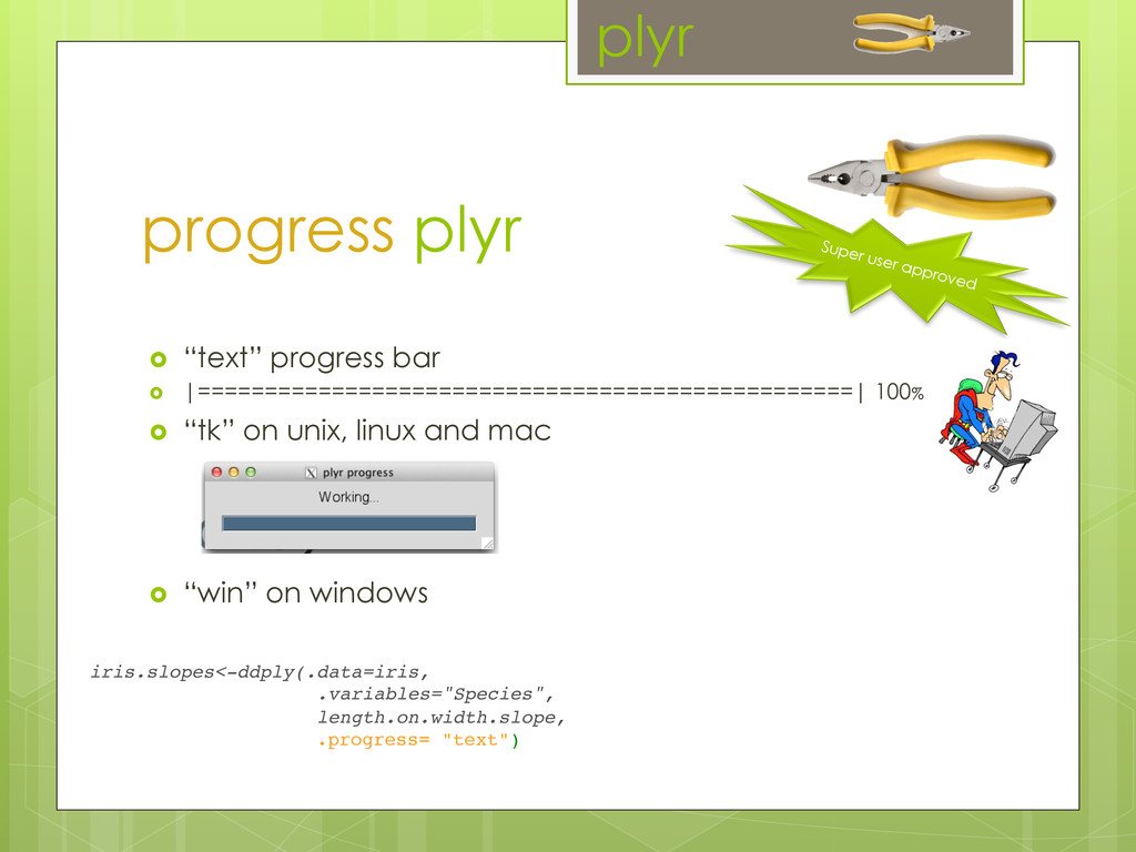
-plyr: split/apply/combine (extract the slope of a linear model for each of your thousand replicates)

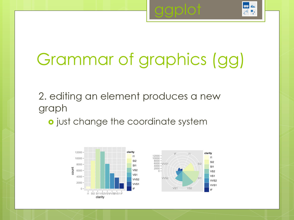
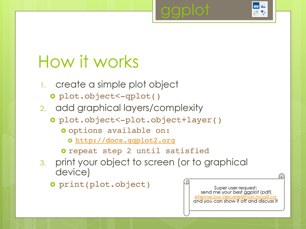
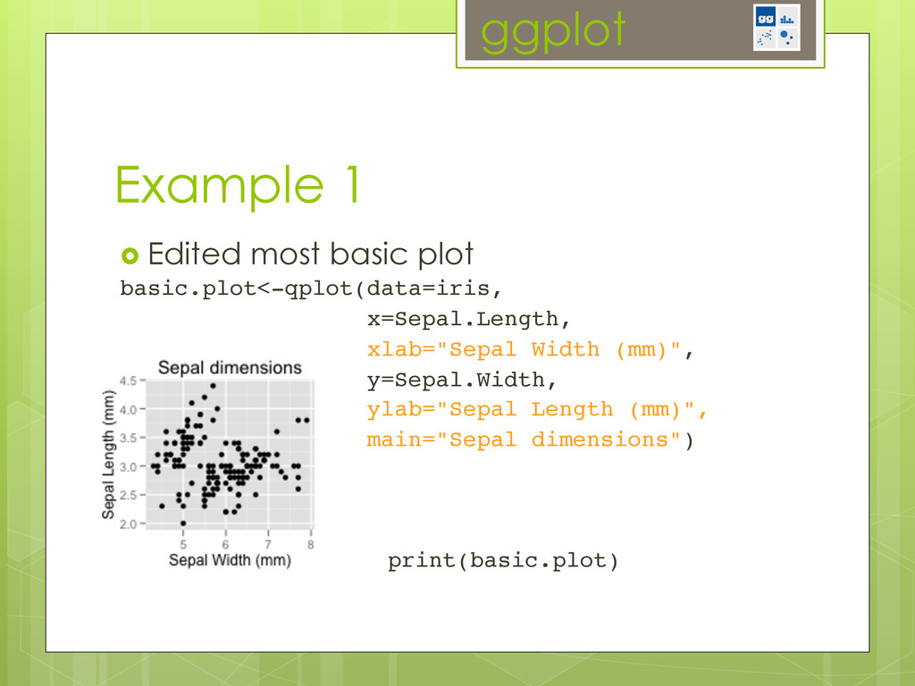
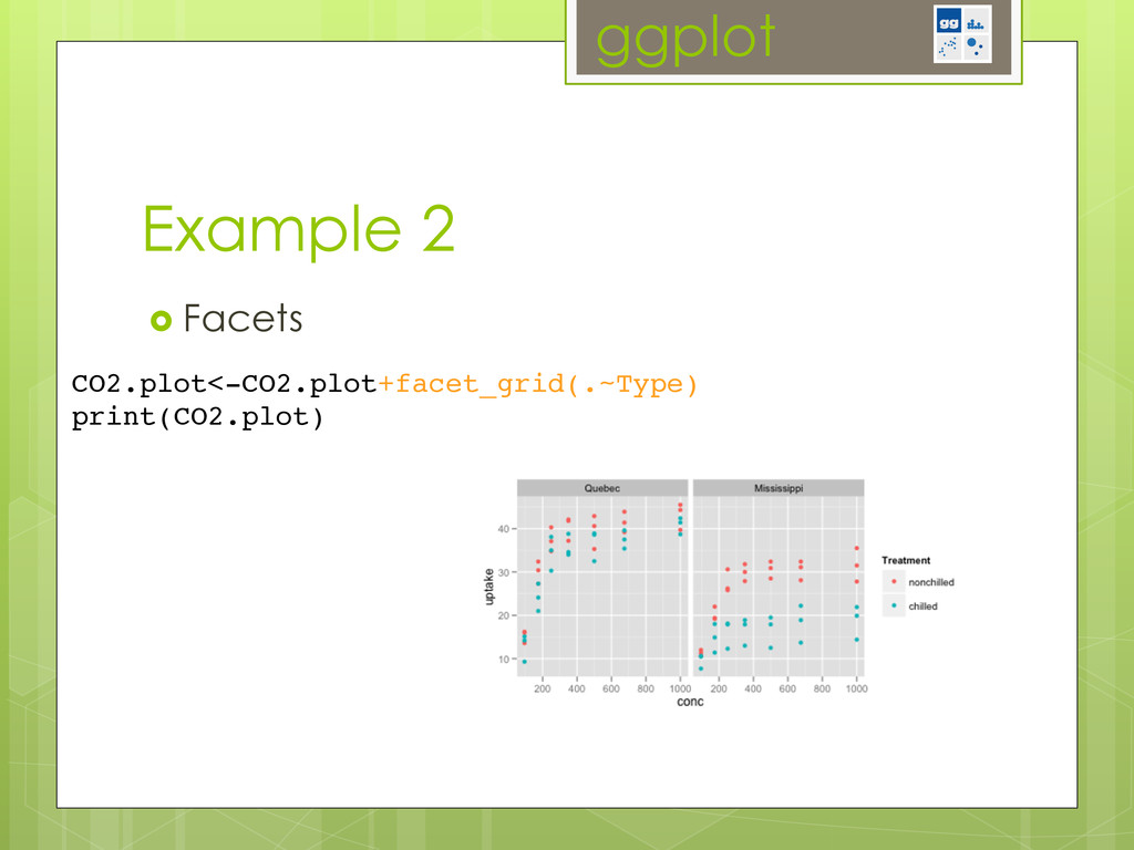
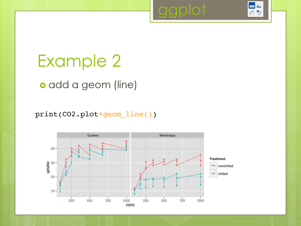
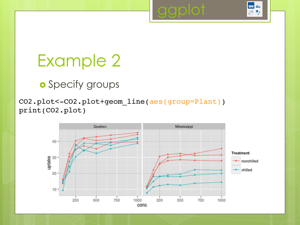
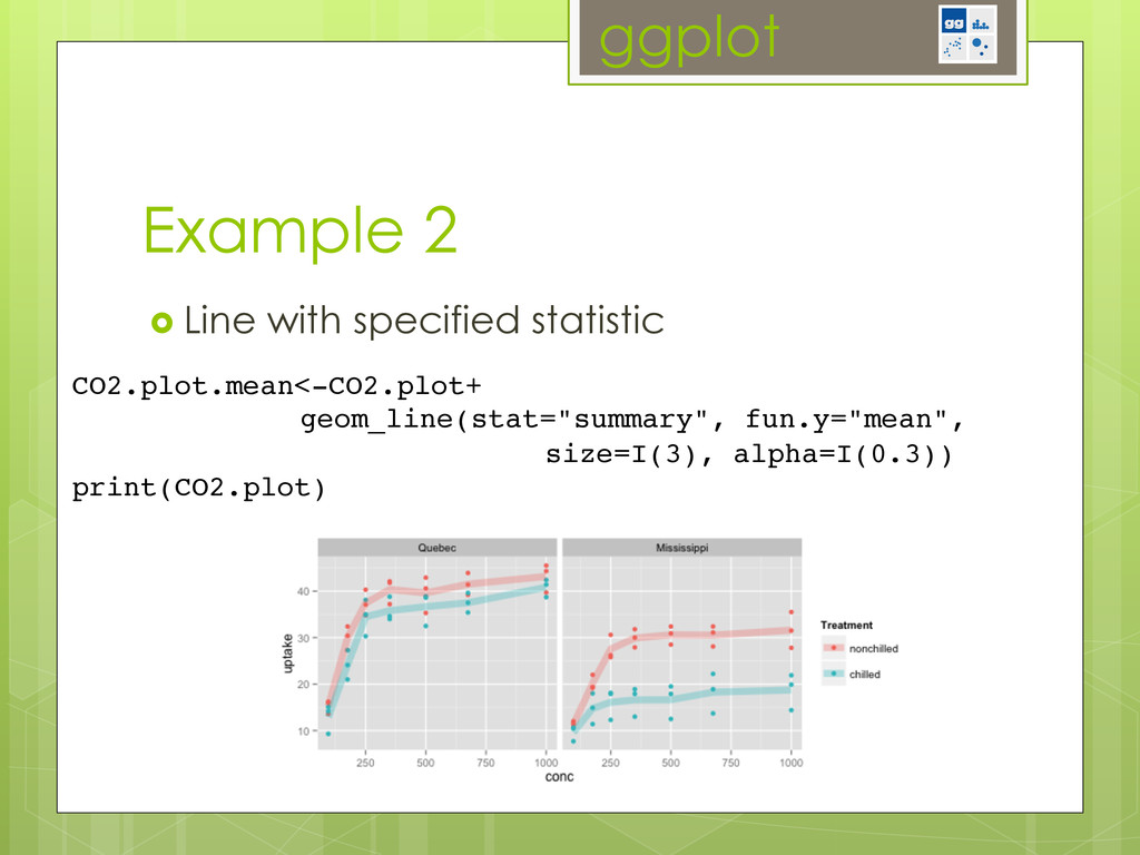
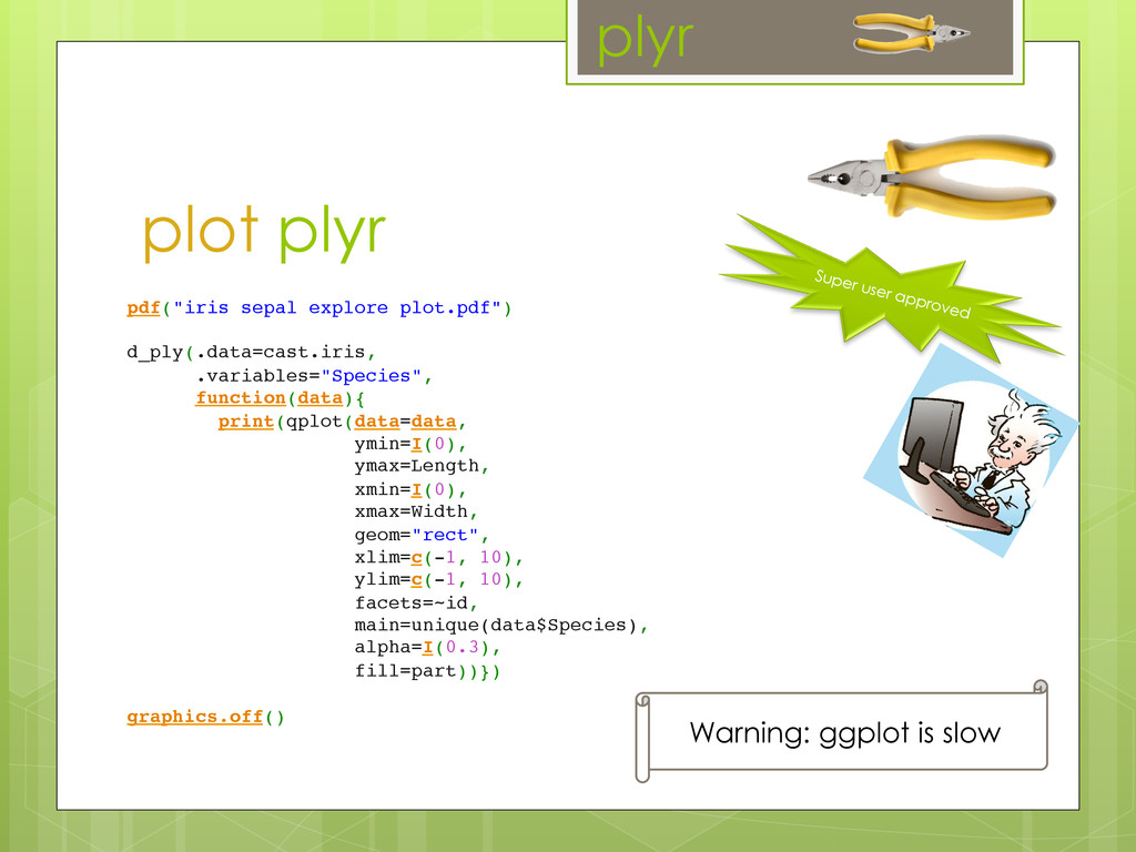
-ggplot2: the grammar of graphics (start with a basic plot and intuitively add layers of complexity)

Transcript

1. The Hadley
   Ecosystem:
   reshape
   plyr
   ggplot
   Etienne Low-Decarie
   Journal of Statistical Software
   7
   2
   1
   1
   2
   1,2
   Figure
   1: T
   he
   three
   ways to
   split up
   a
   2d
   m
   atrix, labelled
   above
   by
   the
   dim
   ensions that they
   slice.
   O
   riginal m
   atrix
   show
   n
   at
   top
   left, w
   ith
   dim
   ensions
   labelled.
   A
   single
   piece
   under
   each
   splitting
   schem
   e
   is
   colored
   blue.
   3
   2
   1
   1
   2
   3
   1,2
   1,3
   2,3
   1,2,3
   Figure
   2:
   T
   he
   seven
   ways
   to
   split
   up
   a
   3d
   array, labelled
   above
   by
   the
   dim
   ensions
   that
   they
   slice
   up.
   O
   riginal array
   show
   n
   at
   top
   left, w
   ith
   dim
   ensions
   labelled.
   Blue
   indicates
   a
   single
   piece
   of the
   output.
   m*ply()
   takes a
   m
   atrix, list-array, or data
   fram
   e, splits it up
   by
   row
   s and
   calls the
   processing
   function
   supplying
   each
   piece
   as
   its
   param
   eters.
   Figure
   3
   show
   s
   how
   you
   m
   ight
   use
   this
   to
   draw
   random
   num
   bers
   from
   norm
   al distributions
   w
   ith
   varying
   param
   eters.
   Input:
   D
   ata
   fram
   e
   (d*ply)
   W
   hen
   operating
   on
   a
   data
   fram
   e, you
   usually
   want
   to
   split
   it
   up
   into
   groups
   based
   on
   com
   -
   binations
   of
   variables
   in
   the
   data
   set.
   For
   d*ply
   you
   specify
   w
   hich
   variables
   (or
   functions
   of variables)
   to
   use.
   T
   hese
   variables
   are
   specified
   in
   a
   special way
   to
   highlight
   that
   they
   are
   

   View Slide

2. goud
   engelhardt
   windmill
   george
   maxine
   corey
   arthur
   rollert
   tanya
   ziegler
   rudolph
   gillis
   tang
   kathryn
   labrecque
   friesen
   caroline
   adekpoe
   tyler
   nicolas
   peika
   brianne
   limberger
   paul
   krause
   moshyk
   julia
   sims
   chapados
   demarsh
   denis
   haller
   caitlin
   charpentier
   surprenant
   kyle
   eric
   sylvain
   cao
   alexandra
   rob
   romana
   romain
   andriy
   colin
   gauthier
   evans
   nick
   miller
   zofia
   yinan
   martins
   jacob
   sacha
   murphy
   heather
   benjamin
   winegardner
   taranu
   ben
   pedersen
   alex
   haine
   ellie
   amanda
   white
   morrison
   chivers
   gibb
   seng
   sumenr
   You
   

   View Slide

3. 0
   50
   100
   Aberdeen
   Austin, TX
   Calgary, AB
   Campinas
   C..te Saint−Luc, QC
   Edinburgh
   Lasalle, QC
   Laval, QC
   Mississauga, ON
   Montreal, QC
   Montr..al, QC
   Montr..al−Ouest, QC
   New York, NY
   Ottawa, ON
   Outremont, QC
   Palo Alto, CA
   Sainte−Julie, QC
   Stowe, VT
   Toronto, ON
   Verdun, QC
   Washington, DC
   Location
   count
   attendee FALSE TRUE
   You
   

   View Slide

4. 0
   20
   40
   60
   0 2 4 6
   RSVPed.Yes
   count
   attendee FALSE TRUE
   You
   

   View Slide

5. You
   ›  R level?
   ›  Have plotted with base R?
   ›  Have you:
   ›  used reshape ?
   ›  used plyr ?
   ›  used ggplot?
   You
   

   View Slide

6. Outline
   ›  reshape
   ›  Make your data play nice
   ›  10 minutes hands on
   ›  plyr
   ›  Split-Apply-Combine on steroids
   ›  to summarize or transform your data
   ›  15 minutes hands on
   ›  ggplot
   ›  beautiful plots one layer at a time
   ›  15 minutes hands on
   ›  Power user goodies on demand
   

   View Slide

7. on demand during hands on:
   superuser stuff
   › ggplot themes
   › plyr
   ›  multicore
   ›  progress bar
   › reshape, plyr and ggplot all together
   ›  great exploratory plots
   › upcoming dplyr
   › more of the Hadely ecosystem
   Journal of Statistical Software
   7
   2
   1
   1
   2
   1,2
   Figure
   1: T
   he
   three
   ways to
   split up
   a
   2d
   m
   atrix, labelled
   above
   by
   the
   dim
   ensions that they
   slice.
   O
   riginal m
   atrix
   show
   n
   at
   top
   left, w
   ith
   dim
   ensions
   labelled.
   A
   single
   piece
   under
   each
   splitting
   schem
   e
   is
   colored
   blue.
   3
   2
   1
   1
   2
   3
   1,2
   1,3
   2,3
   1,2,3
   Figure
   2:
   T
   he
   seven
   ways
   to
   split
   up
   a
   3d
   array, labelled
   above
   by
   the
   dim
   ensions
   that
   they
   slice
   up.
   O
   riginal array
   show
   n
   at
   top
   left, w
   ith
   dim
   ensions
   labelled.
   Blue
   indicates
   a
   single
   piece
   of the
   output.
   m*ply()
   takes a
   m
   atrix, list-array, or data
   fram
   e, splits it up
   by
   row
   s and
   calls the
   processing
   function
   supplying
   each
   piece
   as
   its
   param
   eters.
   Figure
   3
   show
   s
   how
   you
   m
   ight
   use
   this
   to
   draw
   random
   num
   bers
   from
   norm
   al distributions
   w
   ith
   varying
   param
   eters.
   Input:
   D
   ata
   fram
   e
   (d*ply)
   W
   hen
   operating
   on
   a
   data
   fram
   e, you
   usually
   want
   to
   split
   it
   up
   into
   groups
   based
   on
   com
   -
   binations
   of
   variables
   in
   the
   data
   set.
   For
   d*ply
   you
   specify
   w
   hich
   variables
   (or
   functions
   of variables)
   to
   use.
   T
   hese
   variables
   are
   specified
   in
   a
   special way
   to
   highlight
   that
   they
   are
   

   View Slide

8. Follow along
   ›  Code and HTML available at:
   ›  https://github.com/MontrealRUserGroup
   ›  Workshops/Hadley_ecosystem
   

   View Slide

9. Required packages
   ›  the obvious:
   ›  plyr
   ›  reshape(2)
   ›  ggplot2
   ›  for a little more data to play with:
   ›  vegan
   ›  vegetarian
   ›  for pretty graphic tables
   ›  gridExtra
   ›  help(package=“package name”)
   

   View Slide

10. reshape
    reshape
    

    View Slide

11. reshape
    ›  Wide
    ›  Each level of a factor gets a column
    ›  Multiple measurements per row
    ›  Excel, SPSS…
    ›  Pros
    ›  Plays nice with humans
    ›  No data repetition
    ›  “Eyeballable”
    ›  Cons
    ›  Does not play nice with R
    ID variable Level 1 Level 2
    ID 1 Measured value Measured value
    ID 2 Measured value Measured value
    

    View Slide

12. ›  Long
    ›  Levels are expressed in a column
    ›  One measured value per row
    ›  eg. really long: XML, JSON (tag:content pairs)
    ›  Pros
    ›  Plays nice with computers (API, databases, plyr,
    ggplot2…)
    ›  Cons
    ›  Does not play nice with humans
    ›  Lots of copy pasting and forget eyeballing it!
    ID variable Factor Measured value
    ID 1 Level 1 Measured value
    ID 1 Level 2 Measured value
    ID 2 Level 1 Measured value
    ID 2 Level 2 Measured value
    reshape
    

    View Slide

13. Look at data
    ›  What format is…?
    ›  data(simesants)
    ›  head(simesants) or str(simesants)
    ›  data(iris)
    ›  data(sipoo)
    ›  your data???
    ›  Look at more data
    ›  data()
    reshape
    why is your data
    long/wide?
    

    View Slide

14. ID variable Factor Measured value
    ID 1 Level 1 Measured value
    ID 1 Level 2 Measured value
    ID 2 Level 1 Measured value
    ID 2 Level 2 Measured value
    ID variable Level 1 Level 2
    ID 1 Measured value Measured value
    ID 2 Measured value Measured value
    Wide
    Long
    reshape
    

    View Slide

15. Make your data play nice
    ›  Switching from long to wide
    ›  library(reshape)
    ›  melt()
    ›  cast()
    reshape
    

    View Slide

16. Melt: go long
    molten.dataid.vars=ls("id.var.1", "id.var.2"),  
    measure.vars=ls("measure.vars", "measure.vars"),  
    variable_name = "variable")!
    !
    head(iris)  
     
     
     
    reshape
    Super user hint: produce beautiful
    tables with require(gridExtra) and
    grid.table()
    

    View Slide

17. Melt: go long
     
    iris$id  
    molten.irisid.vars=c("Species", "id"),  
    #measure.vars=c("measure.vars", "measure.vars"),  
    variable_name = "measure")  
     
    head(molten.iris)  
     
     
     
    reshape
    

    View Slide

18. Cast: go wide
    cast.dataformula = id_var_1 + id_var_2 ~  
    measure_var_1 + measure_var_2)!
    !
    … means all other variables  
     
     
       
    Super user hint: skip plyr and summarize
    your data with incomplete formula and
    cast(fun.aggregate=…)
    reshape
    

    View Slide

19. Cast: go wide
     
     
    cast.irisformula = Species + id ~ ...)  
     
    head(cast.iris)  
       
    Super user hint: skip plyr and summarize
    your data with incomplete formula and
    cast(fun.aggregate=…)
    reshape
    

    View Slide

20. Your turn
    ›  Try melt and cast
    ›  with baseball produce ->
    ›  with iris: produce:
    reshape
    Discuss how you format/store your data
    with your neighbor
    

    View Slide

21. plyr
    plyr
    

    View Slide

22. plyr
    Plyr
    easily avoid dreaded for loops
    

    View Slide

23. Split-Apply-Combine
    ›  Equivalent
    ›  SQL GROUP BY
    ›  Pivot Tables (Excel, SPSS, …)
    ›  Split
    ›  Define a subset of your data
    ›  Apply
    ›  Do anything to this subset
    ›  calculation, modeling, simulations, plotting
    ›  Combine
    ›  Repeat this for all subsets
    ›  collect the results
    Journal of Statistical Software
    7
    2
    1
    1
    2 1,2
    Figure 1: The three ways to split up a 2d matrix, labelled above by the dimensions that they
    slice. Original matrix shown at top left, with dimensions labelled. A single piece under each
    splitting scheme is colored blue.
    3
    2
    1
    1 2 3
    1,2 1,3 2,3
    1,2,3
    Figure 2: The seven ways to split up a 3d array, labelled above by the dimensions that they
    slice up. Original array shown at top left, with dimensions labelled. Blue indicates a single
    piece of the output.
    m*ply() takes a matrix, list-array, or data frame, splits it up by rows and calls the processing
    function supplying each piece as its parameters. Figure 3 shows how you might use this to
    draw random numbers from normal distributions with varying parameters.
    Input: Data frame (d*ply)
    When operating on a data frame, you usually want to split it up into groups based on com-
    binations of variables in the data set. For d*ply you specify which variables (or functions
    of variables) to use. These variables are specified in a special way to highlight that they are
    Split
    plyr
    

    View Slide

24. Functions
    ›  functions
    ›  _ _ ply
    ›  d = data.frame
    ›  a = array
    ›  l = list
    ›  special
    ›  _ = discard
    ›  r = replicate
    ddply
    input format output format
    plyr
    Super user hint:
    check out help(package=plyr) for
    things like each, join, colwise..
    

    View Slide

25. my.function! ! ! resultsreturn(data.frame(results)}!
    !
    my.function can produce as many rows as subset.data (transform)
    or fewer rows than subset.data (summarize)
    !
    returned.results.variable=c("variable1", "variable2”),!
    ! ! my.function(subset.data))!
    !
    !
    How it works
    Super user hint:
    •  look under the hood as plyr is
    written in R
    •  think you can do better: plyr is
    on GitHub
    Warning: idiosyncrasies
    present
    plyr
    

    View Slide

26. Example 1
    ›  Calculate the mean of each measure for
    each species using the molten data set
    Super user hint: note __ply’s helper
    function rbind.fill() very useful for
    merging many data.frames
    molten.means!.variables=c("Species", "measure"),!
    function(subset.data) data.frame(mean=mean(subset.data$value)))  
    plyr
    

    View Slide

27. Example 3
    ›  Slope of width on length
    Super user hint: on big jobs, plyr can
    tell you where its at (.progress=“text”)
    we can talk about that
    plyr
    length.on.width.slopewith(subset.data,{
    slope.sepalslope.petalreturn(data.frame(slope.sepal=slope.sepal,
    slope.petal=slope.petal))
    })
    }
    iris.slopes.variables="Species",
    function(x)length.on.width.slope(x))
    

    View Slide

28. Your turn
    ›  try mean calculation on original iris
    ›  create different outputs
    ›  dlply
    ›  daply
    ›  d_ply
    ›  when would you use this?
    ›  take in different inputs
    ›  ldply
    ›  rdply
    ›  change functions
    ›  sd, length
    ›  range=max()-min()
    ›  write your own function
    ›  to calculate many statistics
    ›  to do more complex stuff
    ›  calculate slope and intercept of Sepal.Width~Sepal.Length
    ›  to plot
    ›  apply to other data
    ›  melt and cast data
    ›  simesants, rats, iris, sipoo, weeds, your own data
    plyr
    Show your neighbor
    how you would/
    have used plyr
    

    View Slide

29. ggplot
    ggplot
    

    View Slide

30. 6 H. WICKHAM
    Figure 1. Graphics objects produced by (from left to right): geometric objects, scales and coordinate system,
    plot annotations.
    ggplot
    1. a graphic is made of (independent)
    elements layers (as opposed to a single
    encapsulating name)
    ›  data
    ›  aesthetics
    ›  transformation
    ›  geoms (geometric objects)
    ›  axis (coordinate system)
    ›  scales
    Grammar of graphics (gg)
    

    View Slide

31. ggplot
    2. editing an element produces a new
    graph
    ›  just change the coordinate system!
    Grammar of graphics (gg)
    A LAYERED GRAMMAR OF GRAPHICS 23
    Figure 16. Bar chart (left) and equivalent Coxcomb plot (right) of clarity distribution. The Coxcomb plot is a
    bar chart in polar coordinates. Note that the categories abut in the Coxcomb, but are separated in the bar chart:
    this is an example of a graphical convention that differs in different coordinate systems.
    

    View Slide

32. ggplot
    1.  create a simple plot object
    ›  plot.object2.  add graphical layers/complexity
    ›  plot.object›  options available on:!
    ›  http://docs.ggplot2.org!
    ›  repeat step 2 until satisfied!
    3.  print your object to screen (or to graphical
    device)
    ›  print(plot.object)!
    How it works
    Super user request:
    send me your best ggplot (pdf)
    etienne.low-decarie@mail.mcgill.ca
    and you can show it off and discuss it
    

    View Slide

33. ggplot
    Example 1
    ›  Most basic plot
    basic.plotx=Sepal.Length,!
    y=Sepal.Width)!
    !
    ! ! !print(basic.plot)!
    

    View Slide

34. ggplot
    Example 1
    ›  Most basic plot (categorical)
    categorical.plotx=Species,!
    y=Sepal.Width)!
    !
    ! ! !print(categorical.plot)
    

    View Slide

35. ggplot
    Example 1
    ›  Edited most basic plot
    basic.plotx=Sepal.Length,!
    xlab="Sepal Width (mm)",!
    y=Sepal.Width,!
    ylab="Sepal Length (mm)",!
    main="Sepal dimensions")!
    !
    !
    !
    ! ! !print(basic.plot)
    

    View Slide

36. ggplot
    Example 1
    ›  Add aesthetics
    basic.plotx=Sepal.Length,!
    xlab="Sepal Width (mm)",!
    y=Sepal.Width,!
    ylab="Sepal Length (mm)",!
    main="Sepal dimensions",!
    colour=Species,!
    shape=Species,!
    alpha=I(0.5))!
    !
    print(basic.p!
    ! ! !print(basic.plot)!
    

    View Slide

37. ggplot
    Example 1
    ›  Add a geom (eg. linear smooth)
    plot.with.linear.smoothprint(plot.with.linear.smooth)!
    

    View Slide

38. ggplot
    Example 2
    CO2.plotx=conc,!
    y=uptake,!
    colour=Treatment)!
    !
    print(CO2.plot)!
    

    View Slide

39. ggplot
    Example 2
    ›  Facets
    CO2.plotprint(CO2.plot)!
    

    View Slide

40. ggplot
    Example 2
    ›  add a geom (line)
    print(CO2.plot+geom_line())!
    

    View Slide

41. ggplot
    Example 2
    ›  Specify groups
    CO2.plotprint(CO2.plot)!
    

    View Slide

42. ggplot
    Example 2
    ›  Line with specified statistic
    CO2.plot.mean! !geom_line(stat="summary", fun.y="mean",!
    ! ! ! ! size=I(3), alpha=I(0.3))!
    print(CO2.plot)!
    

    View Slide

43. Your turn
    docs.ggplot.org
    ggplot
    Time to show off!
    Show your neighbor the
    prettiest plot you ever
    made!
    http://chrisladroue.com/2011/10/an-exercise-in-plyr-and-ggplot2-using-triathlon-results/
    ›  base
    ›  use data(simeants) ->
    ›  advanced
    ›  use http://chrisladroue.com/files/stratford.csv
    ›  to produce :
    

    View Slide

44. You
    ›  What was most interesting/
    useful?
    ›  What do you still need to
    ›  use reshape, plyr, ggplot?
    ›  to have fun using R?
    

    View Slide

45. Acknowledgements
    ›  Reshape, plyr and ggplot2 are all brought to you on
    GitHub by:
    ›  Hadley Wickham
    ›  had.co.nz
    Wickham, H. (2011). "The split-apply-
    combine strategy for data analysis."
    Journal of Statis.
    Wickham, H. (2010). "A layered
    grammar of graphics." Journal of
    Computational and Graphical
    Statistics 19(1): 3-28.
    

    View Slide

46. Superuser stuff
    ›  ggplot themes
    ›  plyr
    ›  multicore
    ›  progress bar
    ›  reshape, plyr and ggplot all together
    ›  great exploratory plots
    ›  upcoming dplyr
    ›  more of the Hadely ecosystem
    Super user approved
    plyr
    Journal of Statistical Software
    7
    2
    1
    1
    2
    1,2
    Figure
    1: T
    he
    three
    ways to
    split up
    a
    2d
    m
    atrix, labelled
    above
    by
    the
    dim
    ensions that they
    slice.
    O
    riginal m
    atrix
    show
    n
    at
    top
    left, w
    ith
    dim
    ensions
    labelled.
    A
    single
    piece
    under
    each
    splitting
    schem
    e
    is
    colored
    blue.
    3
    2
    1
    1
    2
    3
    1,2
    1,3
    2,3
    1,2,3
    Figure
    2:
    T
    he
    seven
    ways
    to
    split
    up
    a
    3d
    array, labelled
    above
    by
    the
    dim
    ensions
    that
    they
    slice
    up.
    O
    riginal array
    show
    n
    at
    top
    left, w
    ith
    dim
    ensions
    labelled.
    Blue
    indicates
    a
    single
    piece
    of the
    output.
    m*ply()
    takes a
    m
    atrix, list-array, or data
    fram
    e, splits it up
    by
    row
    s and
    calls the
    processing
    function
    supplying
    each
    piece
    as
    its
    param
    eters.
    Figure
    3
    show
    s
    how
    you
    m
    ight
    use
    this
    to
    draw
    random
    num
    bers
    from
    norm
    al distributions
    w
    ith
    varying
    param
    eters.
    Input:
    D
    ata
    fram
    e
    (d*ply)
    W
    hen
    operating
    on
    a
    data
    fram
    e, you
    usually
    want
    to
    split
    it
    up
    into
    groups
    based
    on
    com
    -
    binations
    of
    variables
    in
    the
    data
    set.
    For
    d*ply
    you
    specify
    w
    hich
    variables
    (or
    functions
    of variables)
    to
    use.
    T
    hese
    variables
    are
    specified
    in
    a
    special way
    to
    highlight
    that
    they
    are
    

    View Slide

47. ggplot
    ggplot themes
    ›  theme_set(theme())
    ›  or plot+theme()
    ›  themes
    ›  theme_bw()
    ›  theme_grey()
    ›  edit themes
    ›  mytheme theme(plot.title = element_text(colour = "red"))
    ›  p + mytheme
    

    View Slide

48. multicore plyr
    #install.packages(parallel)!
    #install.packages(doMC)!
    library(parallel)!
    library(doMC)!
    !
    registerDoMC(2) # 2 cores!
    !
    iris.slopes! !.variables="Species",!
    ! !length.on.width.slope,!
    ! !.parallel=T)!
    Super user approved
    plyr
    

    View Slide

49. progress plyr
    ›  “text” progress bar
    ›  |=================================================| 100%
    ›  “tk” on unix, linux and mac
    ›  “win” on windows
    !
    iris.slopes! !.variables="Species",!
    ! !length.on.width.slope,!
    ! !.progress= "text")  
    Super user approved
    plyr
    

    View Slide

50. reshape plyr plot
    Super user approved
    Warning: d_ply is not
    parallel compatible
    1 10 11 12 13 14 15 16
    17 18 19 2 20 21 22 23
    24 25 26 27 28 29 3 30
    31 32 33 34 35 36 37 38
    39 4 40 41 42 43 44 45
    46 47 48 49 5 50 6 7
    8 9
    0
    2
    4
    6
    8
    10
    0
    2
    4
    6
    8
    10
    0
    2
    4
    6
    8
    10
    0
    2
    4
    6
    8
    10
    0
    2
    4
    6
    8
    10
    0
    2
    4
    6
    8
    10
    0
    2
    4
    6
    8
    10
    0 2 4 6 810 0 2 4 6 810
    virginica
    Width
    Length
    part
    Sepal
    Petal
    100 51 52 53 54 55 56 57
    58 59 60 61 62 63 64 65
    66 67 68 69 70 71 72 73
    74 75 76 77 78 79 80 81
    82 83 84 85 86 87 88 89
    90 91 92 93 94 95 96 97
    98 99
    0
    2
    4
    6
    8
    10
    0
    2
    4
    6
    8
    10
    0
    2
    4
    6
    8
    10
    0
    2
    4
    6
    8
    10
    0
    2
    4
    6
    8
    10
    0
    2
    4
    6
    8
    10
    0
    2
    4
    6
    8
    10
    0 2 4 6 810 0 2 4 6 810
    virginica
    Width
    Length
    part
    Sepal
    Petal
    101 102 103 104 105 106 107 108
    109 110 111 112 113 114 115 116
    117 118 119 120 121 122 123 124
    125 126 127 128 129 130 131 132
    133 134 135 136 137 138 139 140
    141 142 143 144 145 146 147 148
    149 150
    0
    2
    4
    6
    8
    10
    0
    2
    4
    6
    8
    10
    0
    2
    4
    6
    8
    10
    0
    2
    4
    6
    8
    10
    0
    2
    4
    6
    8
    10
    0
    2
    4
    6
    8
    10
    0
    2
    4
    6
    8
    10
    0 2 4 6 810 0 2 4 6 810
    virginica
    Width
    Length
    part
    Sepal
    Petal
    plyr
    

    View Slide

51. reshape plyr plot
    Super user approved
    Warning: strsplit is not
    vectorized
    Prepare data using reshape!
    !
    molten.iris$row.namesmolten.iris.variables="row.names",  
    part=unlist(strsplit(x=as.character(measure), split="\\."))[1],  
    dimension=unlist(strsplit(x=as.character(measure), split="\\."))[2],  
    transform)  
     
     
     
    cast.irisformula=Species + id + part ~ dimension)  
    plyr
    

    View Slide

52. plot plyr
    Super user approved
    Warning: ggplot is slow
    pdf("iris sepal explore plot.pdf")  
     
    d_ply(.data=cast.iris,  
    .variables="Species",  
    function(data){  
    print(qplot(data=data,  
    ymin=I(0),  
    ymax=Length,  
    xmin=I(0),  
    xmax=Width,  
    geom="rect",  
    xlim=c(-1, 10),  
    ylim=c(-1, 10),  
    facets=~id,  
    main=unique(data$Species),  
    alpha=I(0.3),  
    fill=part))})  
     
    graphics.off()  
    plyr
    

    View Slide

53. Super user approved
    plyr
    universal plyr:
    coming soon
    dplyr
    data.table[,,]
    

    View Slide

54. ›  devtools: create packages, install
    development versions…
    ›  stringr: easier manipulations of strings
    More from the Hadley
    Ecosystem
    

    View Slide