Upgrade to Pro — share decks privately, control downloads, hide ads and more …

Hash Joins: Past, Present & Future

Hash Joins: Past, Present & Future

A talk I gave about hash joins in PostgreSQL at PGCon 2017 in Ottawa, Canada.
https://www.pgcon.org/2017/schedule/events/1053.en.html
https://www.youtube.com/watch?v=huK-RkxCij8

Thomas Munro

May 25, 2017
Tweet

More Decks by Thomas Munro

Other Decks in Programming

Transcript

  1. About me • EnterpriseDB Database Server team (~ 2 years)

    • PostgreSQL contributions: SKIP LOCKED, remote_apply, replay_lag, DSA (co-author), various smaller things, debugging and review • Relevant active proposal: parallel-aware hash join
  2. Joins • A set of operators from the relational algebra

    • Join operators take two relations and produce a new relation
  3. Example join syntax in SQL • R, S WHERE R.foo

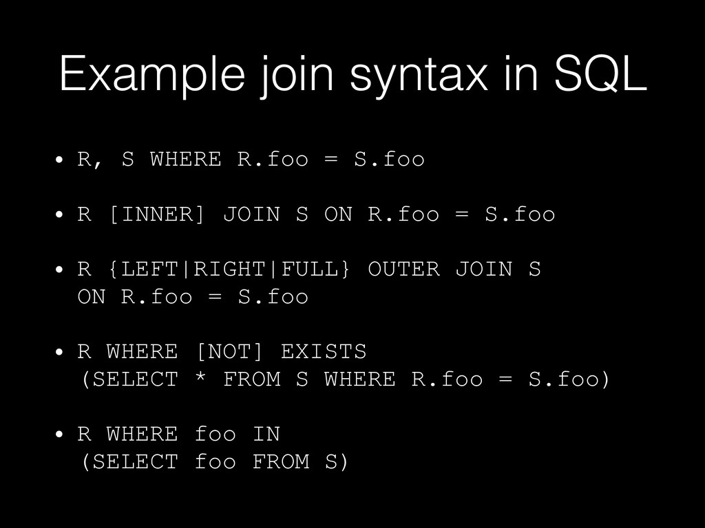
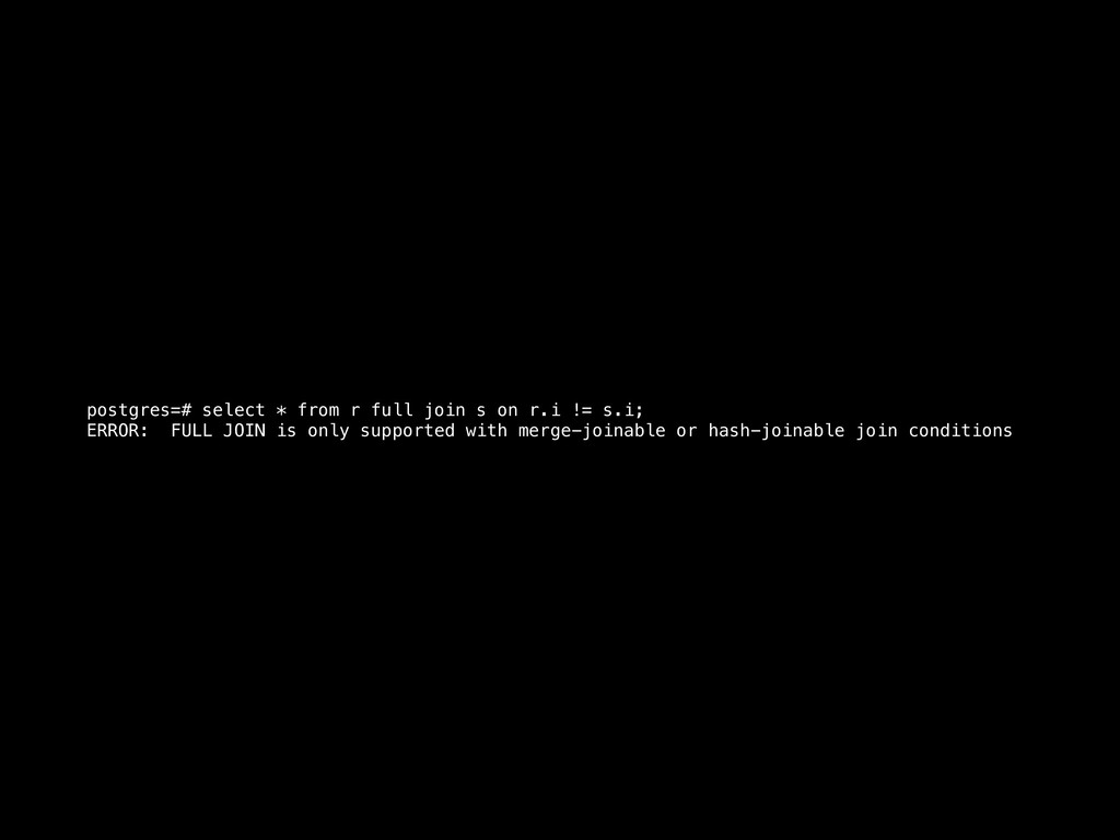
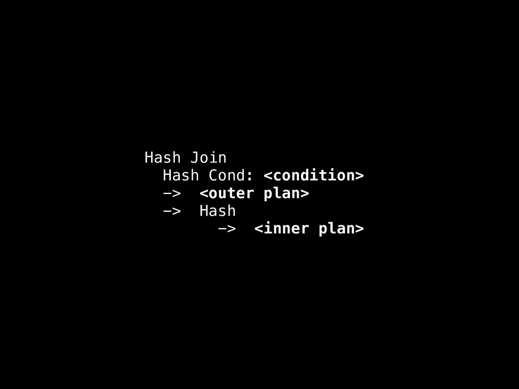
    = S.foo • R [INNER] JOIN S ON R.foo = S.foo • R {LEFT|RIGHT|FULL} OUTER JOIN S
 ON R.foo = S.foo • R WHERE [NOT] EXISTS 
 (SELECT * FROM S WHERE R.foo = S.foo) • R WHERE foo IN 
 (SELECT foo FROM S)
  4. Execution strategies • Nested loop:
 For each tuple in outer

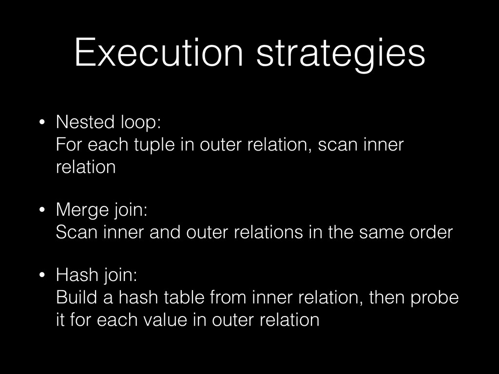
    relation, scan inner relation • Merge join:
 Scan inner and outer relations in the same order • Hash join:
 Build a hash table from inner relation, then probe it for each value in outer relation
  5. M-x squint-mode • A hash join is a bit like

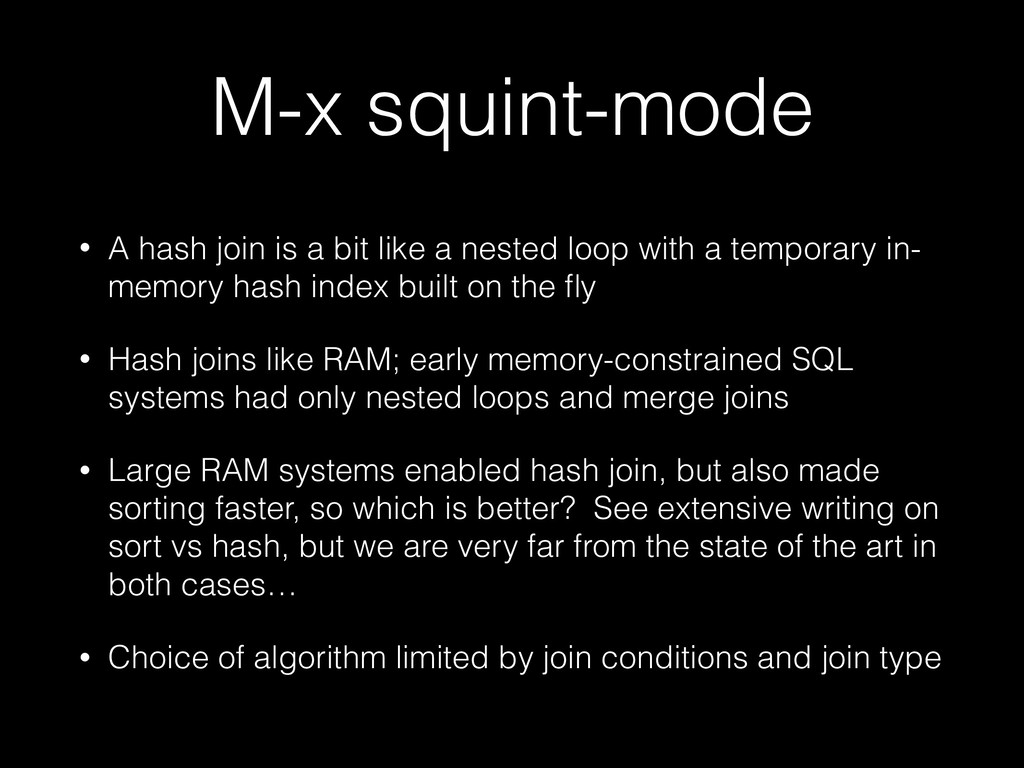
    a nested loop with a temporary in- memory hash index built on the fly • Hash joins like RAM; early memory-constrained SQL systems had only nested loops and merge joins • Large RAM systems enabled hash join, but also made sorting faster, so which is better? See extensive writing on sort vs hash, but we are very far from the state of the art in both cases… • Choice of algorithm limited by join conditions and join type
  6. postgres=# select * from r full join s on r.i

    != s.i; ERROR: FULL JOIN is only supported with merge-joinable or hash-joinable join conditions
  7. Let a hundred
 hash tables bloom • DynaHash: chained (conflict

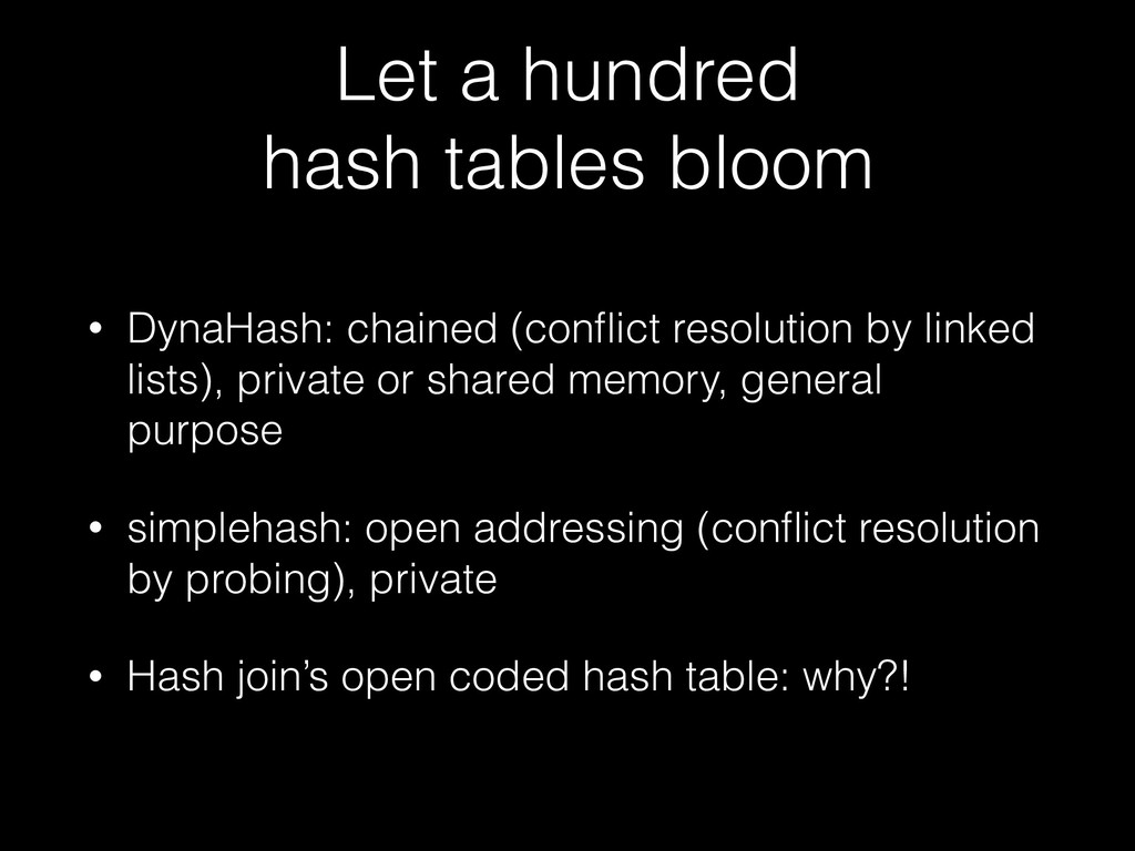
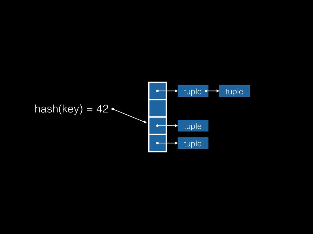
    resolution by linked lists), private or shared memory, general purpose • simplehash: open addressing (conflict resolution by probing), private • Hash join’s open coded hash table: why?!
  8. Hash join table • Little more than an array •

    Multiple tuples with same key (+ unintentional hash collisions); so you’d need to manage your own same-key chain anyway • Hash join has an insert-only phase followed by a read-only probe phase, so very few operations needed • If we need to shrink it due to lack of memory or expand the number of buckets, it’s still the same: free it, allocate a new one and reinsert all the tuples • It’s unclear what would be gained by using one of the other generic implementations: all that is needed is an array!
  9. Chunk-based storage • Tuples are loaded into 32KB chunks, to

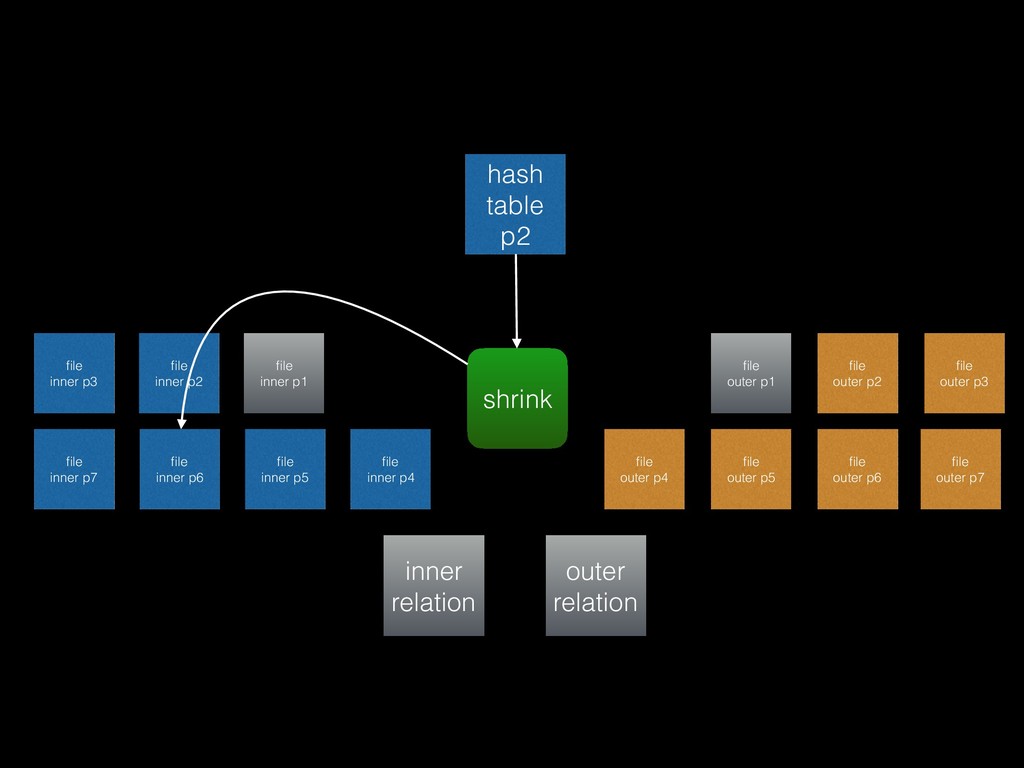
    reduce palloc overhead • This provides a convenient way to iterate over all tuples when we need to resize the bucket array: just replace the array, and loop over all tuples in all chunks reinserting them into the new buckets (= adjusting pointers) • Also useful if we need to dump tuples due to lack of memory: loop over all tuples in all chunks, copying some into new chunks and writing some out to disk
  10. High level algorithm • Build phase: load all the tuples

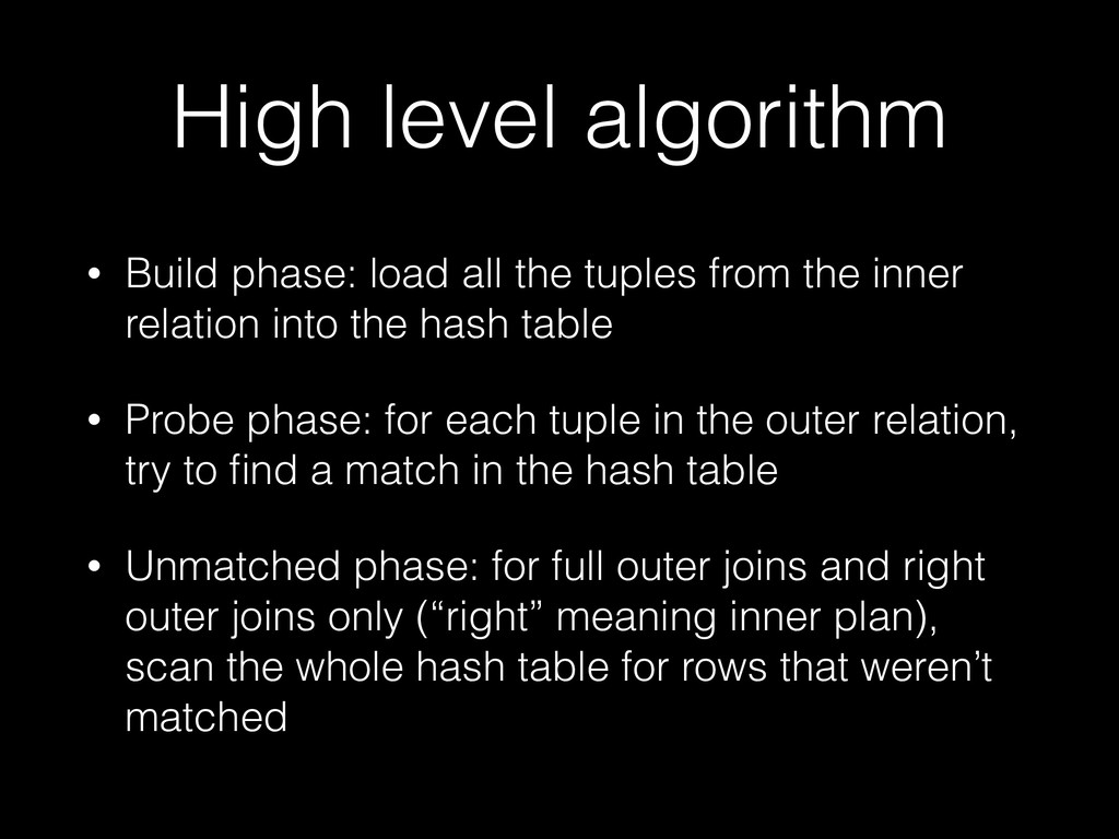
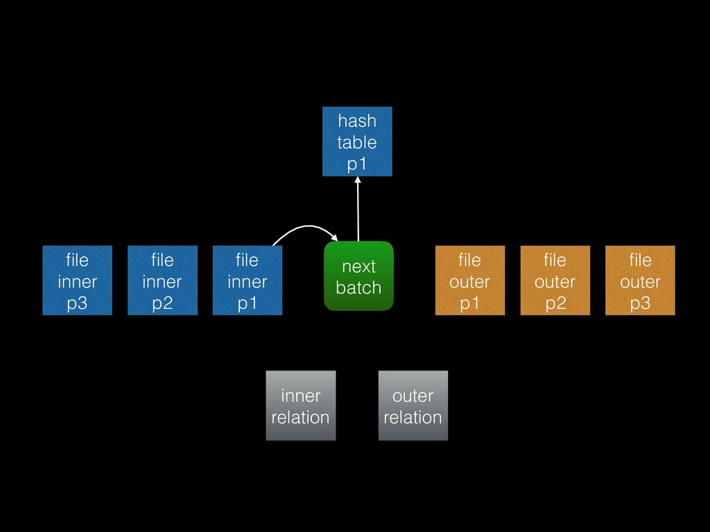
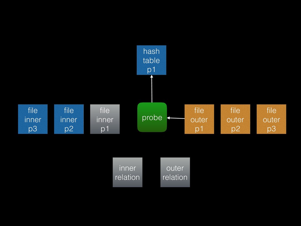
    from the inner relation into the hash table • Probe phase: for each tuple in the outer relation, try to find a match in the hash table • Unmatched phase: for full outer joins and right outer joins only (“right” meaning inner plan), scan the whole hash table for rows that weren’t matched
  11. Optimisations • Empty outer: before attempting to build the hash

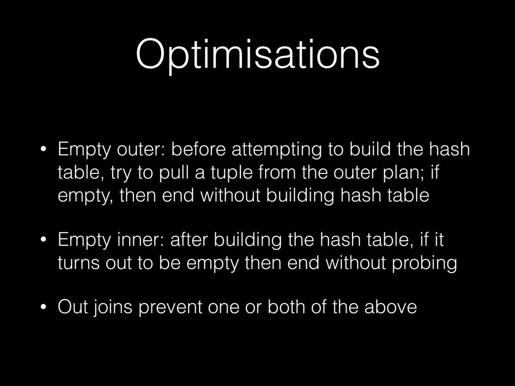
    table, try to pull a tuple from the outer plan; if empty, then end without building hash table • Empty inner: after building the hash table, if it turns out to be empty then end without probing • Out joins prevent one or both of the above
  12. Buckets • Number of tuples* / number of buckets =

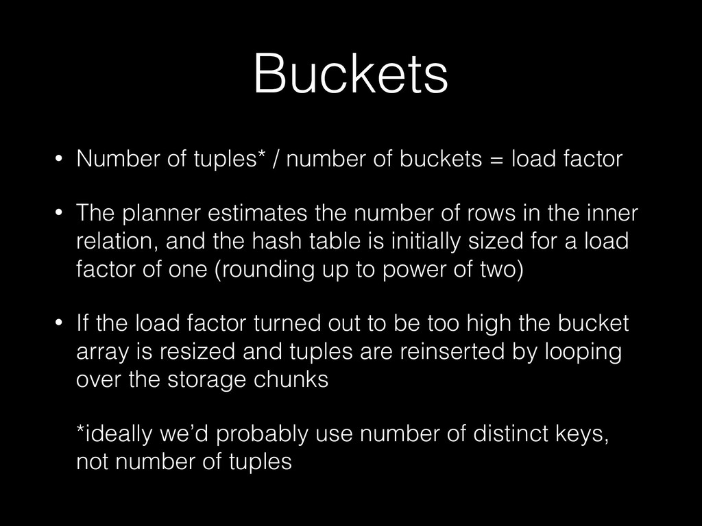
    load factor • The planner estimates the number of rows in the inner relation, and the hash table is initially sized for a load factor of one (rounding up to power of two) • If the load factor turned out to be too high the bucket array is resized and tuples are reinserted by looping over the storage chunks *ideally we’d probably use number of distinct keys, not number of tuples
  13. Hash Join (actual rows=2000 loops=1) Hash Cond: (s.i = r.i)

    -> Seq Scan on s (actual rows=10000 loops=1) -> Hash (actual rows=2000 loops=1) Buckets: 2048 (originally 1024)
 Batches: 1 (originally 1)
 Memory Usage: 87kB -> Seq Scan on r (actual rows=2000 loops=1) Filter: ((i % 5) < 5)
  14. Respecting work_mem • Partition the inner relation into “batches” such

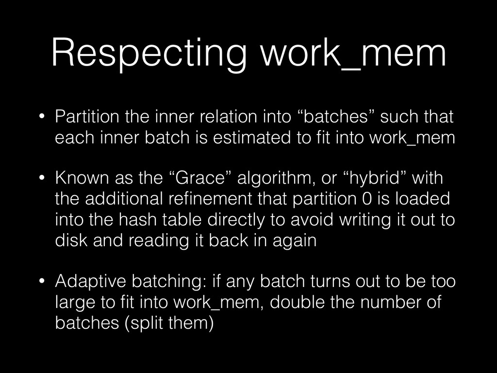
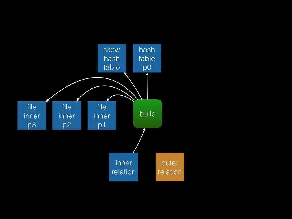
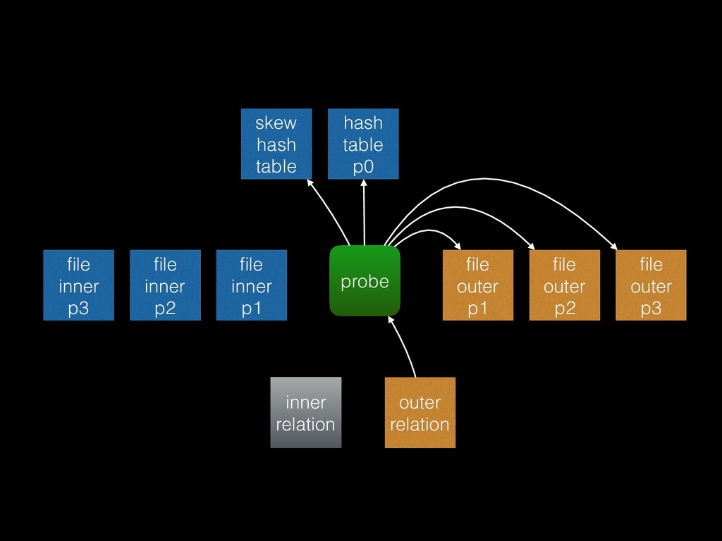
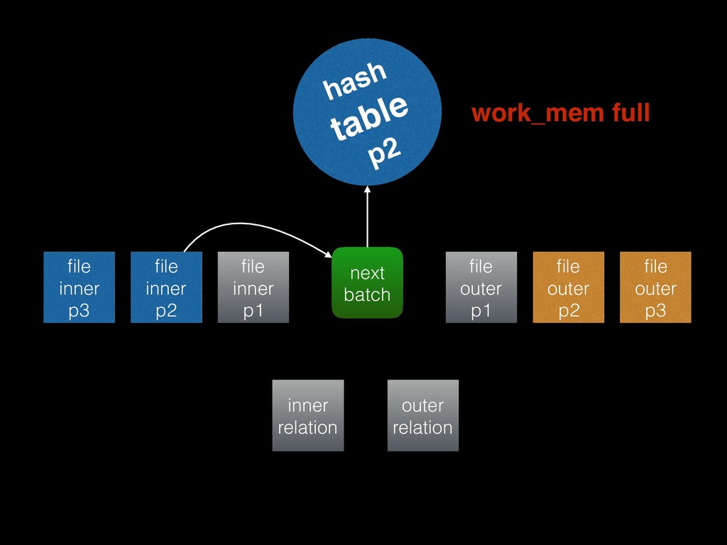
    that each inner batch is estimated to fit into work_mem • Known as the “Grace” algorithm, or “hybrid” with the additional refinement that partition 0 is loaded into the hash table directly to avoid writing it out to disk and reading it back in again • Adaptive batching: if any batch turns out to be too large to fit into work_mem, double the number of batches (split them)
  15. Optimisation • “Skew optimisation”: if the planner determines that we

    should use a multi-batch hash join, then try to use statistics to minimise disk IO. Find the most common values from the outer plan and put matching tuples from the inner plan into special “skew buckets” so that they can be processed as part of partition 0 (ie no disk IO).
  16. hash table
 p0 file inner p1 file inner p2 file

    inner p3 build inner relation outer relation skew hash table
  17. file inner p2 file inner p3 probe inner relation outer

    relation file outer p1 file outer p2 file outer p3 file inner p1 hash table
 p0 skew hash table
  18. file inner p2 file inner p3 next batch inner relation

    outer relation file outer p1 file outer p2 file outer p3 file inner p1 hash table
 p1
  19. file inner p2 file inner p3 probe inner relation outer

    relation file outer p1 file outer p2 file outer p3 file inner p1 hash table
 p1
  20. file inner p2 file inner p3 next batch inner relation

    outer relation file outer p1 file outer p2 file outer p3 file inner p1 hash
 table
 p2 work_mem full
  21. file inner p2 shrink inner relation outer relation file inner

    p1 hash table
 p2 file inner p3 file inner p4 file inner p5 file inner p6 file inner p7 file outer p1 file outer p5 file outer p4 file outer p6 file outer p2 file outer p7 file outer p3
  22. file inner p2 probe inner relation outer relation file inner

    p1 hash table
 p2 file inner p3 file inner p4 file inner p5 file inner p6 file inner p7 file outer p1 file outer p5 file outer p4 file outer p6 file outer p2 file outer p7 file outer p3
  23. Hash join behaviour modes • “Optimal” — the planner thinks

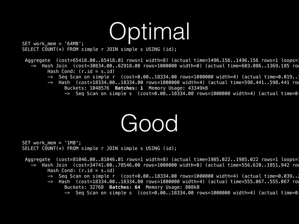
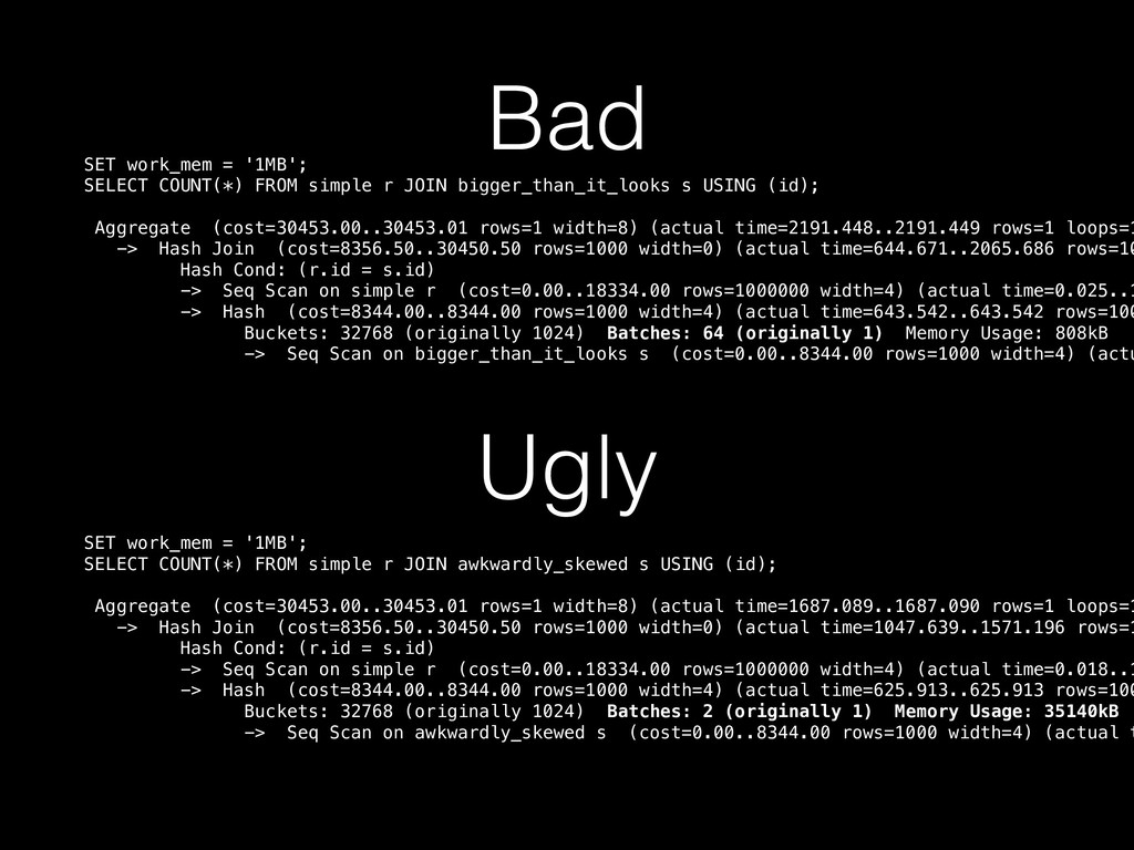
    the hash table will fit in memory, and the executor finds this to be true • “Good” — the planner thinks that N > 1 batches will allow every batch to fit in work_mem, and the executor finds this to be true • “Bad” — as for “optimal” or “good”, but the executor finds that it needs to increase the number of partitions, dumping some of tuples out to disk, and possibly rewriting outer tuples • “Ugly” — as for “bad”, but the executor finds that the data is sufficiently skewed that increasing the number of batches won’t help; it stops respecting work_mem and hopes for the best!
  24. Out of memory: Kill process 1020 (postgres) score 64 or

    sacrifice child Killed process 1020 (postgres) total-vm:445764kB, anon-rss:140640kB, file-rss:136092kB
  25. Optimal SET work_mem = '64MB';
 SELECT COUNT(*) FROM simple r

    JOIN simple s USING (id); Aggregate (cost=65418.00..65418.01 rows=1 width=8) (actual time=1496.156..1496.156 rows=1 loops=1 -> Hash Join (cost=30834.00..62918.00 rows=1000000 width=0) (actual time=603.086..1369.185 row Hash Cond: (r.id = s.id) -> Seq Scan on simple r (cost=0.00..18334.00 rows=1000000 width=4) (actual time=0.019..1 -> Hash (cost=18334.00..18334.00 rows=1000000 width=4) (actual time=598.441..598.441 row Buckets: 1048576 Batches: 1 Memory Usage: 43349kB -> Seq Scan on simple s (cost=0.00..18334.00 rows=1000000 width=4) (actual time=0. Good SET work_mem = '1MB'; SELECT COUNT(*) FROM simple r JOIN simple s USING (id); 
 Aggregate (cost=81046.00..81046.01 rows=1 width=8) (actual time=1985.022..1985.022 rows=1 loops=1 -> Hash Join (cost=34741.00..78546.00 rows=1000000 width=0) (actual time=556.620..1851.942 row Hash Cond: (r.id = s.id) -> Seq Scan on simple r (cost=0.00..18334.00 rows=1000000 width=4) (actual time=0.039..2 -> Hash (cost=18334.00..18334.00 rows=1000000 width=4) (actual time=555.067..555.067 row Buckets: 32768 Batches: 64 Memory Usage: 808kB -> Seq Scan on simple s (cost=0.00..18334.00 rows=1000000 width=4) (actual time=0.
  26. Bad SET work_mem = '1MB';
 SELECT COUNT(*) FROM simple r

    JOIN bigger_than_it_looks s USING (id); Aggregate (cost=30453.00..30453.01 rows=1 width=8) (actual time=2191.448..2191.449 rows=1 loops=1 -> Hash Join (cost=8356.50..30450.50 rows=1000 width=0) (actual time=644.671..2065.686 rows=10 Hash Cond: (r.id = s.id) -> Seq Scan on simple r (cost=0.00..18334.00 rows=1000000 width=4) (actual time=0.025..1 -> Hash (cost=8344.00..8344.00 rows=1000 width=4) (actual time=643.542..643.542 rows=100 Buckets: 32768 (originally 1024) Batches: 64 (originally 1) Memory Usage: 808kB -> Seq Scan on bigger_than_it_looks s (cost=0.00..8344.00 rows=1000 width=4) (actu Ugly SET work_mem = '1MB'; SELECT COUNT(*) FROM simple r JOIN awkwardly_skewed s USING (id); 
 Aggregate (cost=30453.00..30453.01 rows=1 width=8) (actual time=1687.089..1687.090 rows=1 loops=1 -> Hash Join (cost=8356.50..30450.50 rows=1000 width=0) (actual time=1047.639..1571.196 rows=1 Hash Cond: (r.id = s.id) -> Seq Scan on simple r (cost=0.00..18334.00 rows=1000000 width=4) (actual time=0.018..1 -> Hash (cost=8344.00..8344.00 rows=1000 width=4) (actual time=625.913..625.913 rows=100 Buckets: 32768 (originally 1024) Batches: 2 (originally 1) Memory Usage: 35140kB -> Seq Scan on awkwardly_skewed s (cost=0.00..8344.00 rows=1000 width=4) (actual t
  27. Parallel query recap • “Partial plans” are plans that can

    be run by many workers in parallel, so that each will generate a fraction of the total results • Parallel Sequential Scan and Parallel Index Scan nodes emit tuples to the nodes above them using page granularity • Every plan node above such a scan is part of a partial plan, until parallelism is terminated by a Gather or Gather Merge node
  28. Parallel-oblivious hash joins in PostgreSQL 9.6 & 10 • A

    Hash Join node can appear in a partial plan • It is not “parallel aware”, meaning that it isn’t doing anything special to support parallelism: if its outer plan happens to be partial, then its output will also be partial • Problem 1: the inner plan is run in every process, and a copy of the hash table is built in each • Problem 2: since there are multiple hash tables with their own ‘matched’ flags, we can’t allow full or right outer joins to be parallelised
  29. Amdahl’s outlaw • Parallelising the probe phase but not the

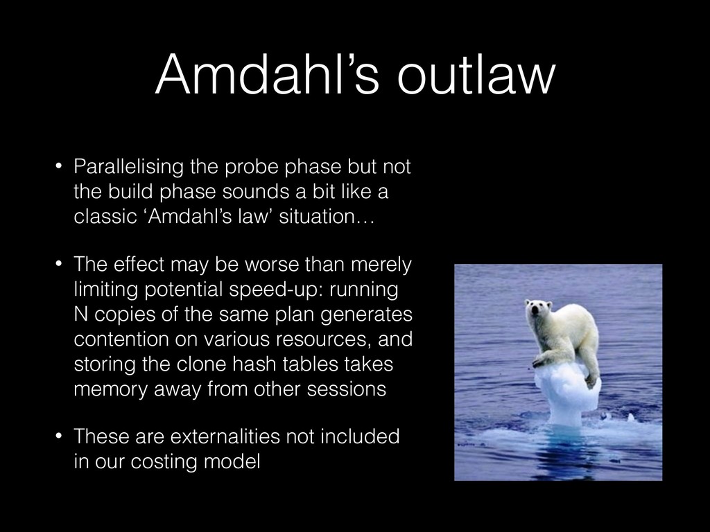
    build phase sounds a bit like a classic ‘Amdahl’s law’ situation… • The effect may be worse than merely limiting potential speed-up: running N copies of the same plan generates contention on various resources, and storing the clone hash tables takes memory away from other sessions • These are externalities not included in our costing model
  30. Which? • Partition-wise joins work with parallel-oblivious join operators, but

    requires the user to have declared suitable partitions • State-of-the-art cache-aware repartitioning algorithm “radix join” adds a costly multi-pass partitioning phase, minimising cache misses during probing • Several researchers claim that a simple shared hash table is usually about as good, and often better in skewed cases[1] [2], despite cache misses; not everyone agrees[3] • The bar for beating a no-partition shared hash table seems very high, in terms of engineering challenges
  31. Proposal: shared hash table • Tuples and hash table stored

    in memory from new ‘DSA’ allocator; special relative pointers must be used • Insertion into buckets using compare-and-swap • Wait for all peers at key points — in common case just end of build, but in multi-batch case more waits — using a ‘barrier’ IPC mechanism • Needs various shared infrastructure: shared memory allocator (DSA), shared temporary files, shared tuplestores, shared record typmod registry, barrier primitive + condition variable • Complications relating to leader process’s dual role
  32. SELECT COUNT(*) FROM simple r JOIN simple s USING (id)

    JOIN simple t USING (id) JOIN simple u USING (id);
  33. Finalize Aggregate (cost=1228093.57..1228093.58 rows=1 width=8) (actual time=24324.455..24324.456 rows= -> Gather

    (cost=1228093.15..1228093.56 rows=4 width=8) (actual time=24010.300..24324.433 rows=5 loop Workers Planned: 4 Workers Launched: 4 -> Partial Aggregate (cost=1227093.15..1227093.16 rows=1 width=8) (actual time=24004.404..2400 -> Hash Join (cost=925007.40..1220843.10 rows=2500020 width=0) (actual time=19254.859..2 Hash Cond: (r.id = u.id) -> Hash Join (cost=616671.60..850006.80 rows=2500020 width=12) (actual time=12700. Hash Cond: (r.id = t.id) -> Hash Join (cost=308335.80..479170.50 rows=2500020 width=8) (actual time=6 Hash Cond: (r.id = s.id) -> Parallel Seq Scan on simple r (cost=0.00..108334.20 rows=2500020 wi -> Hash (cost=183334.80..183334.80 rows=10000080 width=4) (actual time Buckets: 16777216 Batches: 1 Memory Usage: 482635kB -> Seq Scan on simple s (cost=0.00..183334.80 rows=10000080 widt -> Hash (cost=183334.80..183334.80 rows=10000080 width=4) (actual time=6376. Buckets: 16777216 Batches: 1 Memory Usage: 482635kB -> Seq Scan on simple t (cost=0.00..183334.80 rows=10000080 width=4) ( -> Hash (cost=183334.80..183334.80 rows=10000080 width=4) (actual time=6478.513..6 Buckets: 16777216 Batches: 1 Memory Usage: 482635kB -> Seq Scan on simple u (cost=0.00..183334.80 rows=10000080 width=4) (actual Total memory usage = ~500MB * 3 * 5 = ~7.5GB
  34. Finalize Aggregate (cost=607466.61..607466.62 rows=1 width=8) (actual time=11247.154..11247.154 rows=1 -> Gather

    (cost=607466.19..607466.60 rows=4 width=8) (actual time=10998.218..11247.133 rows=5 loops= Workers Planned: 4 Workers Launched: 4 -> Partial Aggregate (cost=606466.19..606466.20 rows=1 width=8) (actual time=10989.275..10989. -> Parallel Hash Join (cost=426256.41..600216.14 rows=2500020 width=0) (actual time=4842 Hash Cond: (r.id = u.id) -> Parallel Hash Join (cost=284170.94..436255.49 rows=2500020 width=12) (actual ti Hash Cond: (r.id = t.id) -> Parallel Hash Join (cost=142085.47..272294.84 rows=2500020 width=8) (actu Hash Cond: (r.id = s.id) -> Parallel Seq Scan on simple r (cost=0.00..108334.20 rows=2500020 wi -> Parallel Shared Hash (cost=108334.20..108334.20 rows=2500020 width= Buckets: 16777216 Batches: 1 Memory Usage: 522336kB -> Parallel Seq Scan on simple s (cost=0.00..108334.20 rows=2500 -> Parallel Shared Hash (cost=108334.20..108334.20 rows=2500020 width=4) (ac Buckets: 16777216 Batches: 1 Memory Usage: 522368kB -> Parallel Seq Scan on simple t (cost=0.00..108334.20 rows=2500020 wi -> Parallel Shared Hash (cost=108334.20..108334.20 rows=2500020 width=4) (actual t Buckets: 16777216 Batches: 1 Memory Usage: 522304kB -> Parallel Seq Scan on simple u (cost=0.00..108334.20 rows=2500020 width=4) Total memory usage = ~500MB * 3 = ~1.5GB
  35. Memory Escape Valve? • If extra rounds of adaptive partitioning

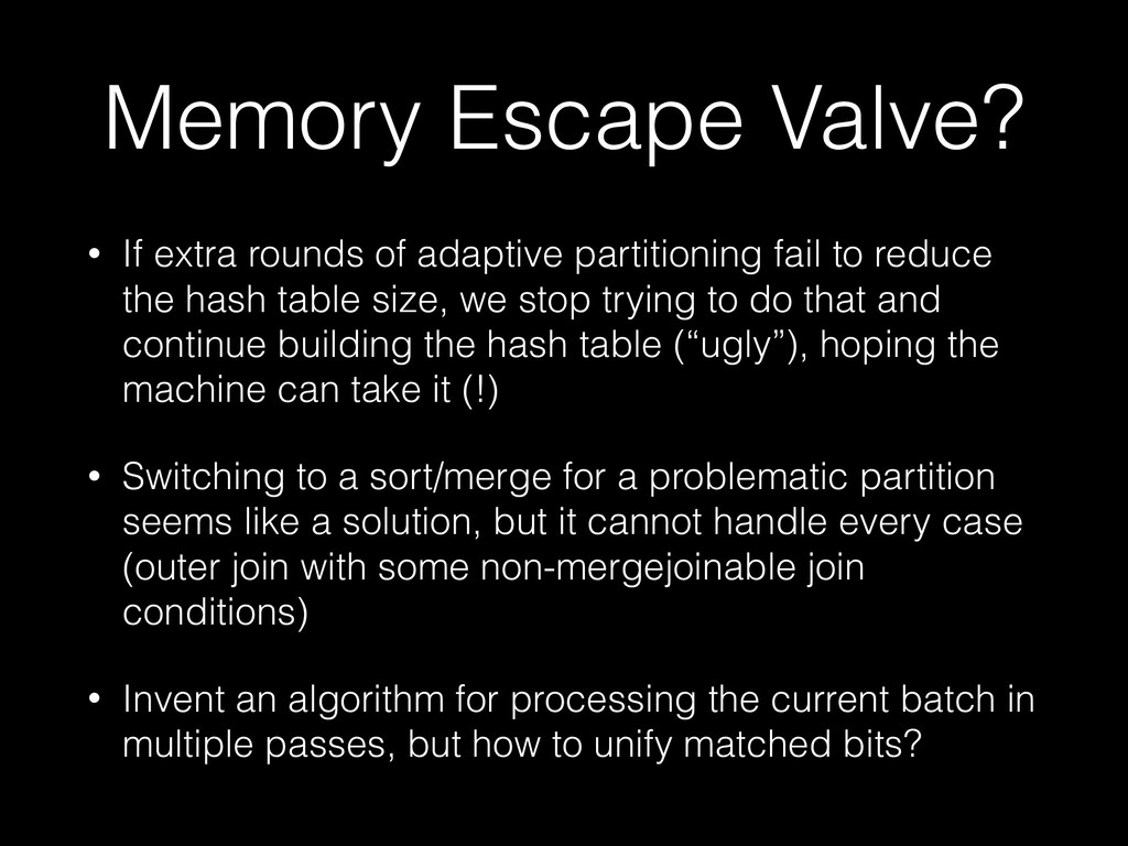
    fail to reduce the hash table size, we stop trying to do that and continue building the hash table (“ugly”), hoping the machine can take it (!) • Switching to a sort/merge for a problematic partition seems like a solution, but it cannot handle every case (outer join with some non-mergejoinable join conditions) • Invent an algorithm for processing the current batch in multiple passes, but how to unify matched bits?
  36. Bloom filters? • Could we profitably push Bloom filters from

    the hash table down to the outer scan? • Could we use Bloom filters to filter the data written to outer relation batch files?
  37. N-join peak memory? join join U join T R S

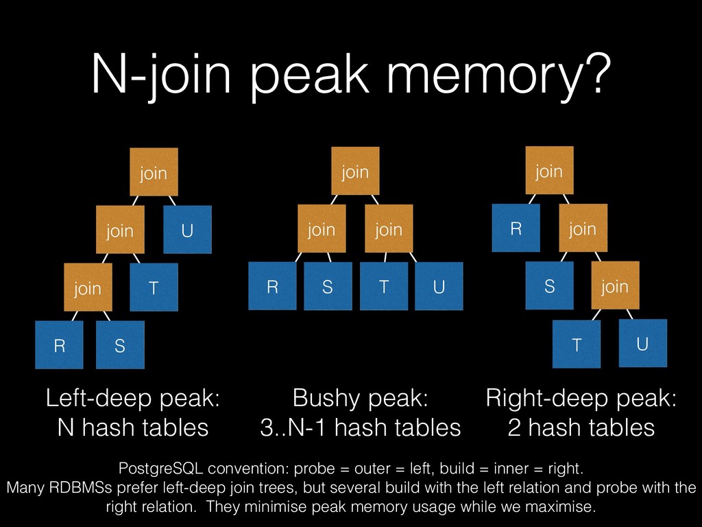
    join join join R S T U join R join join S T U Bushy peak:
 3..N-1 hash tables Left-deep peak:
 N hash tables Right-deep peak:
 2 hash tables PostgreSQL convention: probe = outer = left, build = inner = right. Many RDBMSs prefer left-deep join trees, but several build with the left relation and probe with the right relation. They minimise peak memory usage while we maximise.
  38. Tune chunk size? • We want 32KB but the actual

    size that hits the system malloc, after palloc overhead and chunk header, is 32KB + a smidgen, which eats up to 36KB of real space on some OSes • We should probably make this much bigger to dilute that effect, or tune the size to allow for headers • There may be other reasons to crank up the chunk size
  39. References • [1] Design and Evaluation of Main Memory Hash

    Join Algorithms for Multi-core CPUs, 2011 • [2] Andy Pavlo’s CMU 15-721 2017 lecture “Parallel Join Algorithms (Hashing)”, available on Youtube + slides • [3] Main-Memory Hash Joins on Multi-Core CPUs: Tuning to the Underlying Hardware, 2013