Onia 2013-04-05 meeting

Transcript

1. Status report on χ b production Alexander Mazurov Ferrara University, CERN Onia Production and Polarisation Meeting 2013-04-05
2. 2 Motivation bb system, which can be produced in different spin configurations, is ideal laboratory for QCD tests. ̄ It is like a hydrogen atom in QCD. States with paralell quark spins (S=1): • S-wave ϒ state • P-wave χ b states, composed by 3 spin states χ b(0,1,2) . Can be readily produced in the radiactive decays of ϒ. • χ b (3P) state recently observed by ATLAS, D0 and LHCb Study of χ b production: • Measurement for ϒ(1,2,3S) cross sections in χ b decays as a function of p T (Nϒ) • Measurement of χ b(0,1,3) (3P) mass. • Measured mass • Mass from theory
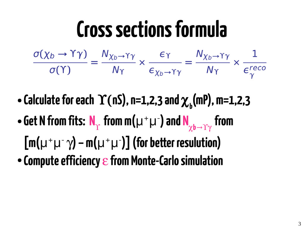
3. 3 Cross sections formula • Calculate for each ϒ(nS), n=1,2,3 and χ b (mP), m=1,2,3 • Get N from fits: N ϒ from m(µ+µ-) and N χb→ϒγ from [m(µ+µ- γ) – m(µ+µ-)] (for better resulution) • Compute efficiency ε from Monte-Carlo simulation
4. 4 In this talk • Updated fit model for mass difference [m(µ+µ- γ) – m(µ+µ-)] • Monte-Carlo validation
5. 5 Datasets • 2011: Luminosity = 1015 ± 35 pb-1 (Vanya 's MDST) (Re)Produced this week: • 2011: Reco14 / Stripping20r1 / WGBandQSelection3 / BOTTOM.MDST • 2012: Reco14 / Stripping20 / WGBandQSelection3 / BOTTOM.MDST
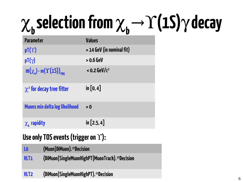
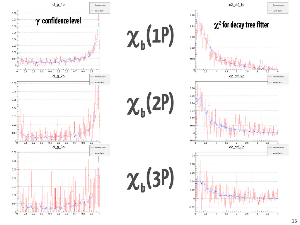
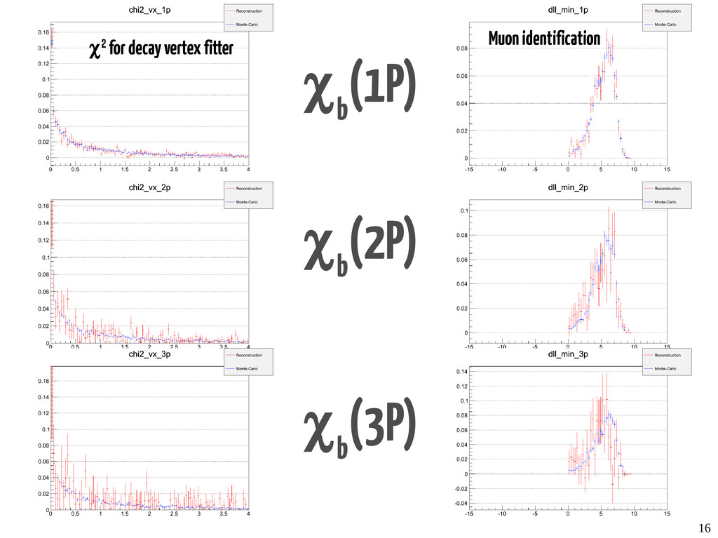
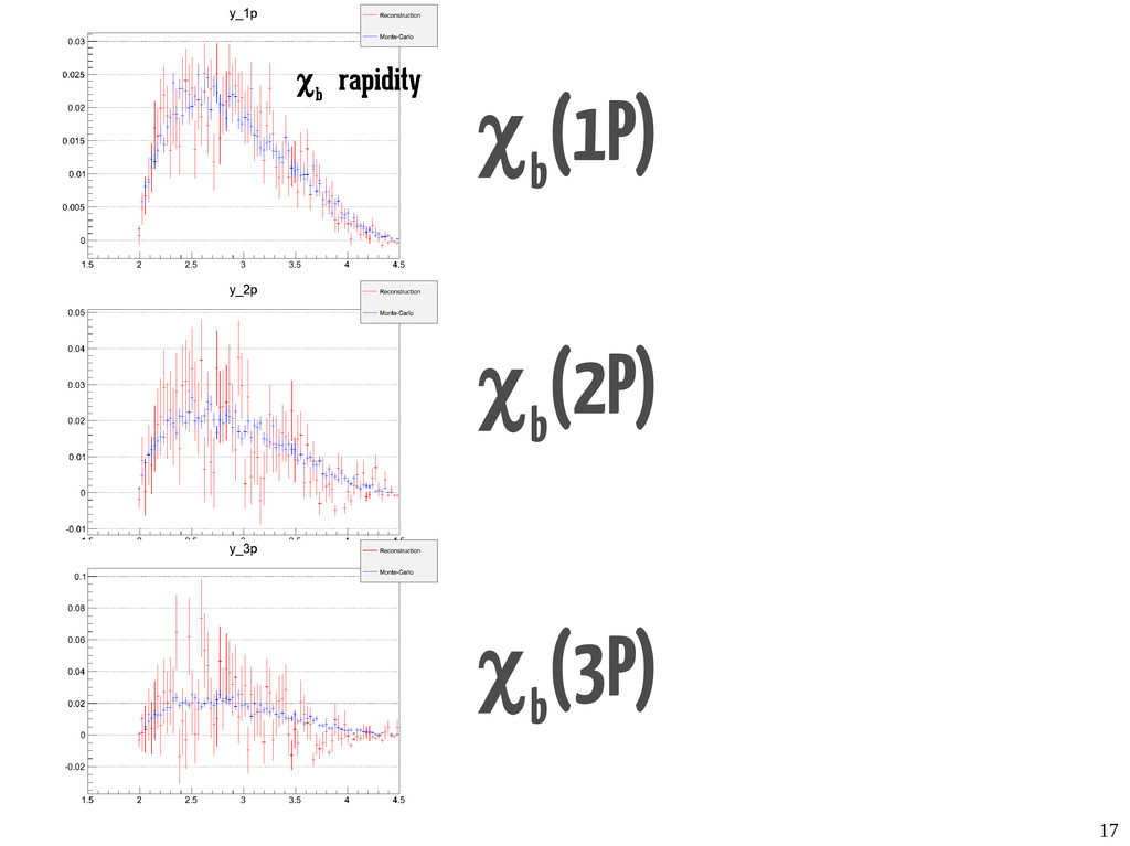
6. 6 χ b selection from χ b →ϒ(1S)γ decay Parameter Values pT(ϒ) > 14 GeV (in nominal fit) pT(γ) > 0.6 GeV m(χ b ) - m(ϒ(1S)) PDG < 0.2 GeV/c2 χ2 for decay tree fitter in [0, 4] Muons min delta log likelihood > 0 χ b rapidity in [2.5, 4] Use only TOS events (trigger on ϒ): L0 (Muon|DiMuon).*Decision HLT1 (DiMuon|SingleMuonHighPT|MuonTrack).*Decision HLT2 (DiMuon|SingleMuonHighPT).*Decision
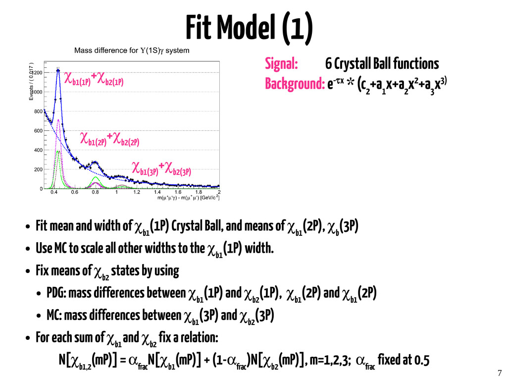
7. 7 Fit Model (1) χ b1(1P) +χ b2(1P) χ b1(2P) +χ b2(2P) χ b1(3P) +χ b2(3P) Signal: 6 Crystall Ball functions Background: e-τx * (c 2 +a 1 x+a 2 x2+a 3 x3) • Fit mean and width of χ b1 (1P) Crystal Ball, and means of χ b1 (2P), χ b (3P) • Use MC to scale all other widths to the χ b1 (1P) width. • Fix means of χ b2 states by using • PDG: mass differences between χ b1 (1P) and χ b2 (1P), χ b1 (2P) and χ b1 (2P) • MC: mass differences between χ b1 (3P) and χ b2 (3P) • For each sum of χ b1 and χ b2 fix a relation: N[χ b1,2 (mP)] = α frac N[χ b1 (mP)] + (1-α frac )N[χ b2 (mP)], m=1,2,3; α frac fixed at 0.5
8. 8 Fit model(2) χ b1(1P) +χ b2(1P) χ b1(2P) +χ b2(2P) χ b1(3P) +χ b2(3P) CB(χ b1(1P) ) floating parameters: mean and width. CB(χ b2(1P) ) no floating parameters; mean = mean(χ b1(1P) ) + delta_mass1 PDG ; width = coeff1 MC * width(χ b1(1P) ) CB(χ b1(2P) ) floating parameters: mean; width = coeff2 MC * width(χ b1(1P) ) CB(χ b2(2P) ) no floating parameters; mean = mean(χ b1(2P) ) + delta_mass2 PDG ; width = coeff3 MC * width(χ b1(2P) ) CB(χ b1(2P) ) floating parameters: mean; width = coeff4 MC * width(χ b1(1P) ) CB(χ b2(2P) ) no floating parameters; mean = mean(χ b1(2P) ) + delta_mass3 MC ; width = coeff5 MC * width(χ b1(2P) ) Background: all 4 parameters are floating (τ, a 1 , a 2 , a 3 ) Number of events: N[χ b(1P) ]: 2954 ± 125 N[χ b(2P) ]: 740 ± 67 N[χ b(3P) ]: 288 ± 48 The significance of the χ b (3P) signal 5.88 sigma
9. 9 Systematic Constraint N[χ b (1P)] change(%) N[χ b (2P)] change(%) N[χ b (3P)] change(%) N[χ b (2P)]/N[χ b (1P)] change(%) N[χ b (3P)]/N[χ b (1P)] change(%) α frac [χ b (1P)] = 0 3 3 3 0 1 α frac [χ b (1P)] = 1 3 3 3 0 1 α frac [χ b (2P)] = 0 2 -2 1 -4 0 α frac [χ b (2P)] = 1 0 -1 0 -1 0 α frac [χ b (3P)] = 0 0 0 -1 0 -1 α frac [χ b (3P)] = 1 0 0 0 0 0 Fix max PDG mass diff between χ b1 (1P) and χ b2 (1P) 2 -4 7 -6 -8 Fix max PDG mass diff between χ b1 (2P) and χ b2 (2P) 0 0 0 0 0 • Systematic uncertainties due to relative contributions of χ b1 and χ b2 states • Other systematic uncertainties are under study.
10. 10 pT(ϒ) spectrum • PT(ϒ) binning: [10 , 11, 12, 14,18,30] • The yields are not divided by the bin width
11. 11 Data vs. MC • Compare decay parameters distribution on data and MC. • Plots for the data parameters obtained by using sPlot technique. • Using the same cuts that shown on χ b selection slide.
12. 12 pT(γ) pT(ϒ) χ b (1P) χ b (2P) χ b (3P)
13. 13 χ b (1P) χ b (2P) χ b (3P) pT(χ b ) min[pT(µ+) ,pT(µ-)]
14. 14 χ b (1P) χ b (2P) χ b (3P) min[p(µ+) , p(µ−)]
15. 15 χ b (1P) χ b (2P) χ b (3P) γ confidence level χ2 for decay tree fitter
16. 16 χ b (1P) χ b (2P) χ b (3P) Muon identification χ2 for decay vertex fitter
17. 17 χ b (1P) χ b (2P) χ b (3P) χ b rapidity
18. 18 Conclusion • Fit model is basically ready. • Due to nice agreement between data and MC we can trust the MC to compute efficiencies. Next: process new 2011 and 2012 data