Coastal vegetation: mangroves, seagrass and saltmarsh as drag, in flow and wave models

Plants are described explicitly by height, density and stem size rather than folded into bed roughness. They act as drag in the flow models and dissipate wave energy in Spectral Waves. The flow results are compared with laboratory flume measurements by Ghisalberti and Nepf (2004). MIKE 21/3 Coupled Model FM and MIKE 21/3 Wave Model FM, since Release 2022.

Transcript

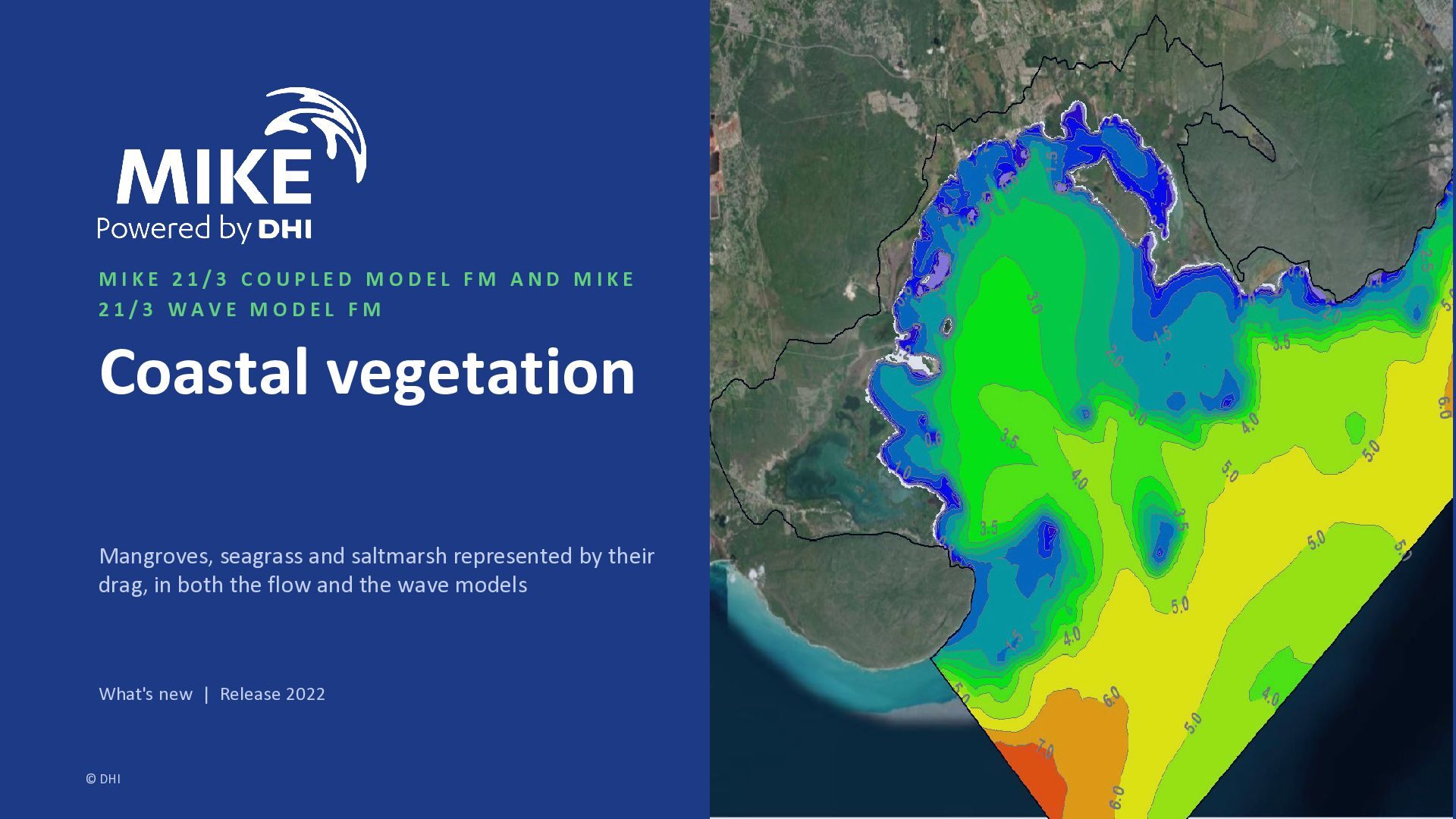
1. MIKE 21/3 COUPLED MODEL FM AND MIKE 21/3 WAVE MODEL FM Coastal vegetation Mangroves, seagrass and saltmarsh represented by their drag, in both the flow and the wave models What's new | Release 2022 © DHI
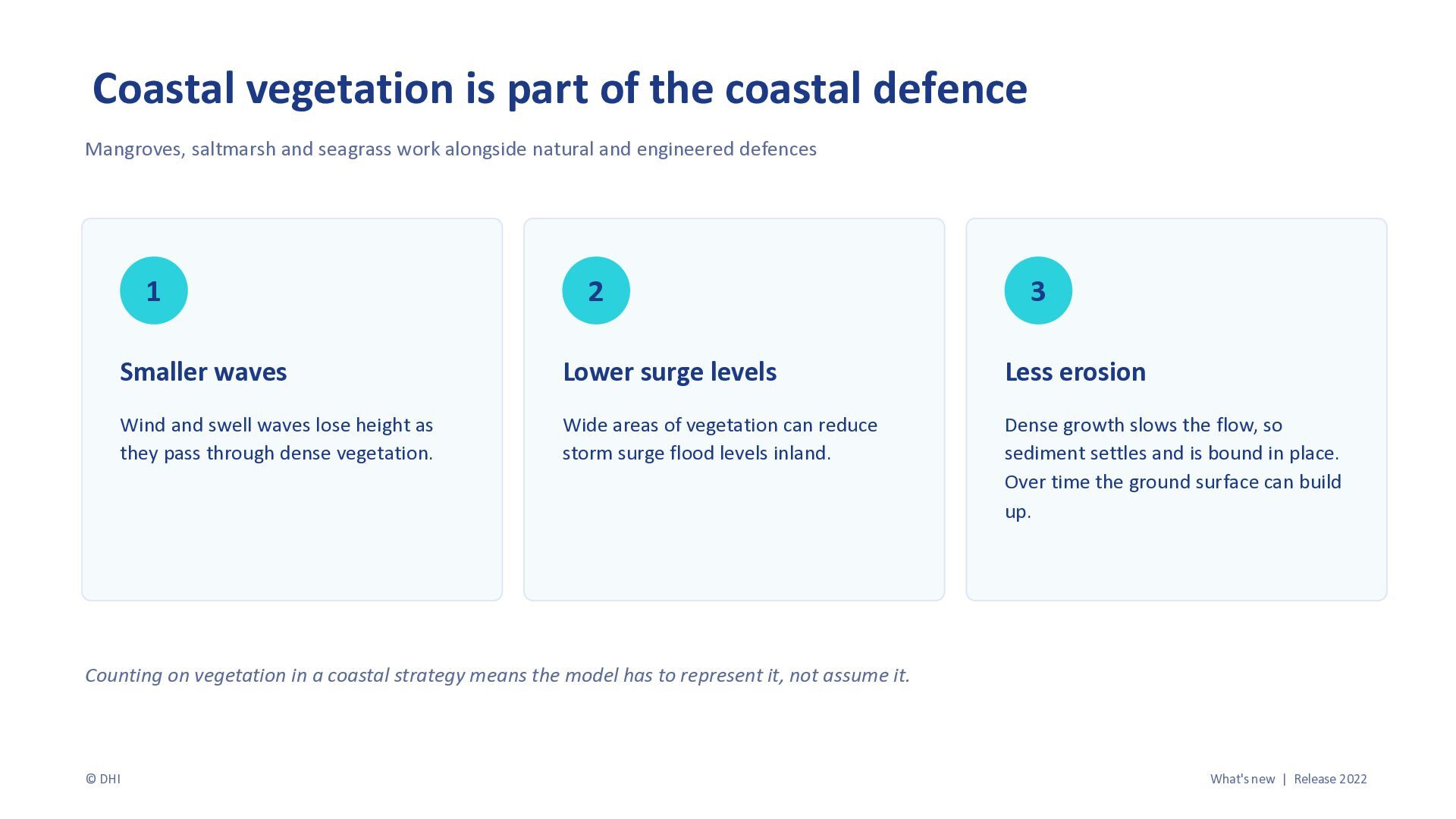
2. Coastal vegetation is part of the coastal defence Mangroves, saltmarsh and seagrass work alongside natural and engineered defences 1 2 3 Smaller waves Lower surge levels Less erosion Wind and swell waves lose height as they pass through dense vegetation. Wide areas of vegetation can reduce storm surge flood levels inland. Dense growth slows the flow, so sediment settles and is bound in place. Over time the ground surface can build up. Counting on vegetation in a coastal strategy means the model has to represent it, not assume it. © DHI What's new | Release 2022
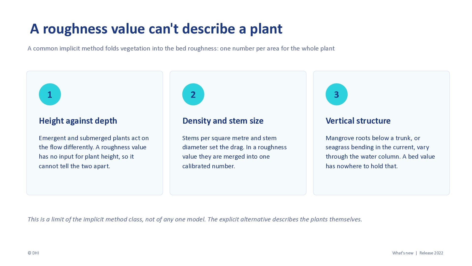
3. A roughness value can't describe a plant A common implicit method folds vegetation into the bed roughness: one number per area for the whole plant 1 2 3 Height against depth Density and stem size Vertical structure Emergent and submerged plants act on the flow differently. A roughness value has no input for plant height, so it cannot tell the two apart. Stems per square metre and stem diameter set the drag. In a roughness value they are merged into one calibrated number. Mangrove roots below a trunk, or seagrass bending in the current, vary through the water column. A bed value has nowhere to hold that. This is a limit of the implicit method class, not of any one model. The explicit alternative describes the plants themselves. © DHI What's new | Release 2022
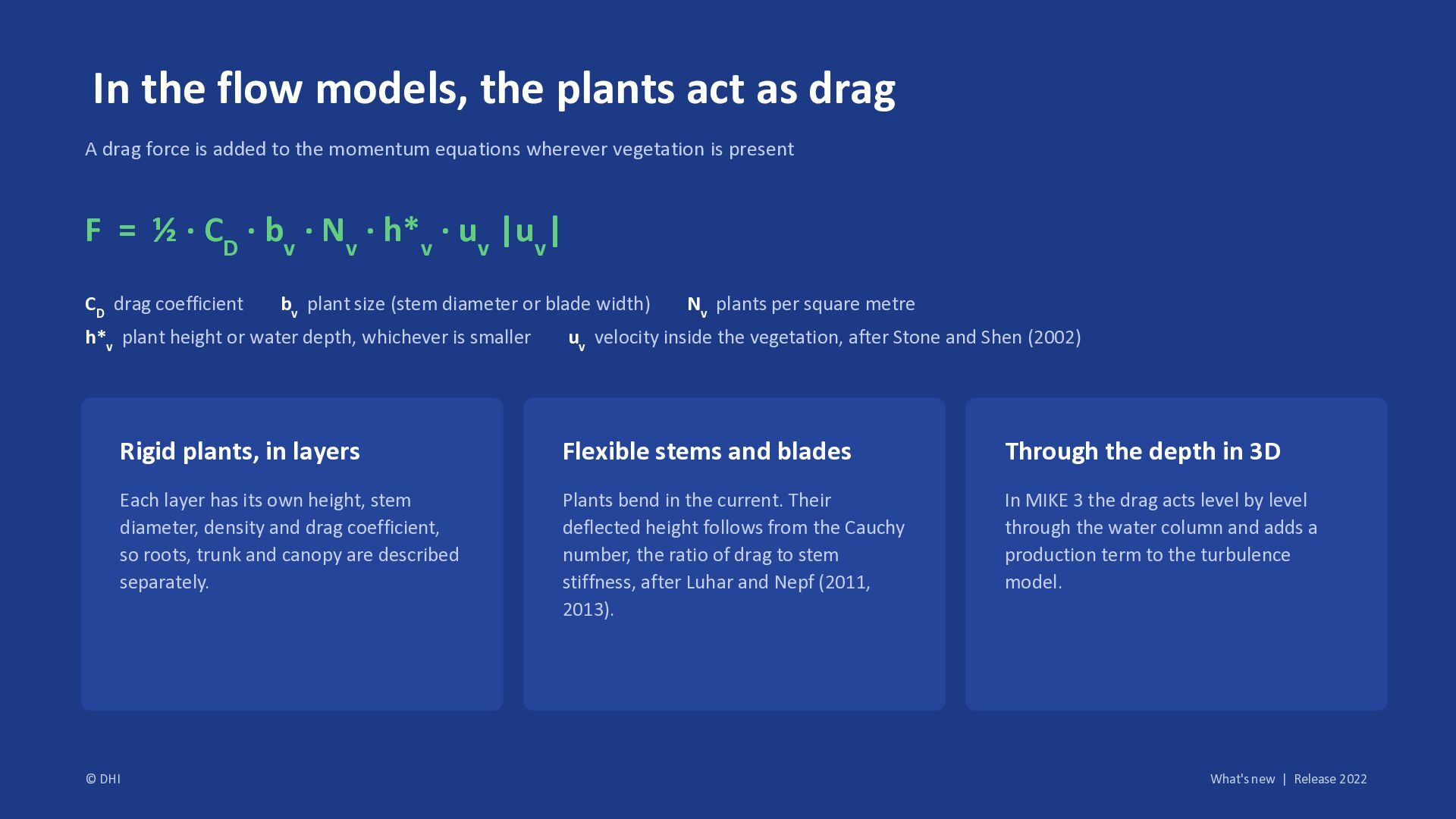
4. In the flow models, the plants act as drag A drag force is added to the momentum equations wherever vegetation is present F = ½ · CD · bv · Nv · h*v · uv |uv| CD drag coefficient bv plant size (stem diameter or blade width) h*v plant height or water depth, whichever is smaller © DHI Nv plants per square metre uv velocity inside the vegetation, after Stone and Shen (2002) Rigid plants, in layers Flexible stems and blades Through the depth in 3D Each layer has its own height, stem diameter, density and drag coefficient, so roots, trunk and canopy are described separately. Plants bend in the current. Their deflected height follows from the Cauchy number, the ratio of drag to stem stiffness, after Luhar and Nepf (2011, 2013). In MIKE 3 the drag acts level by level through the water column and adds a production term to the turbulence model. What's new | Release 2022
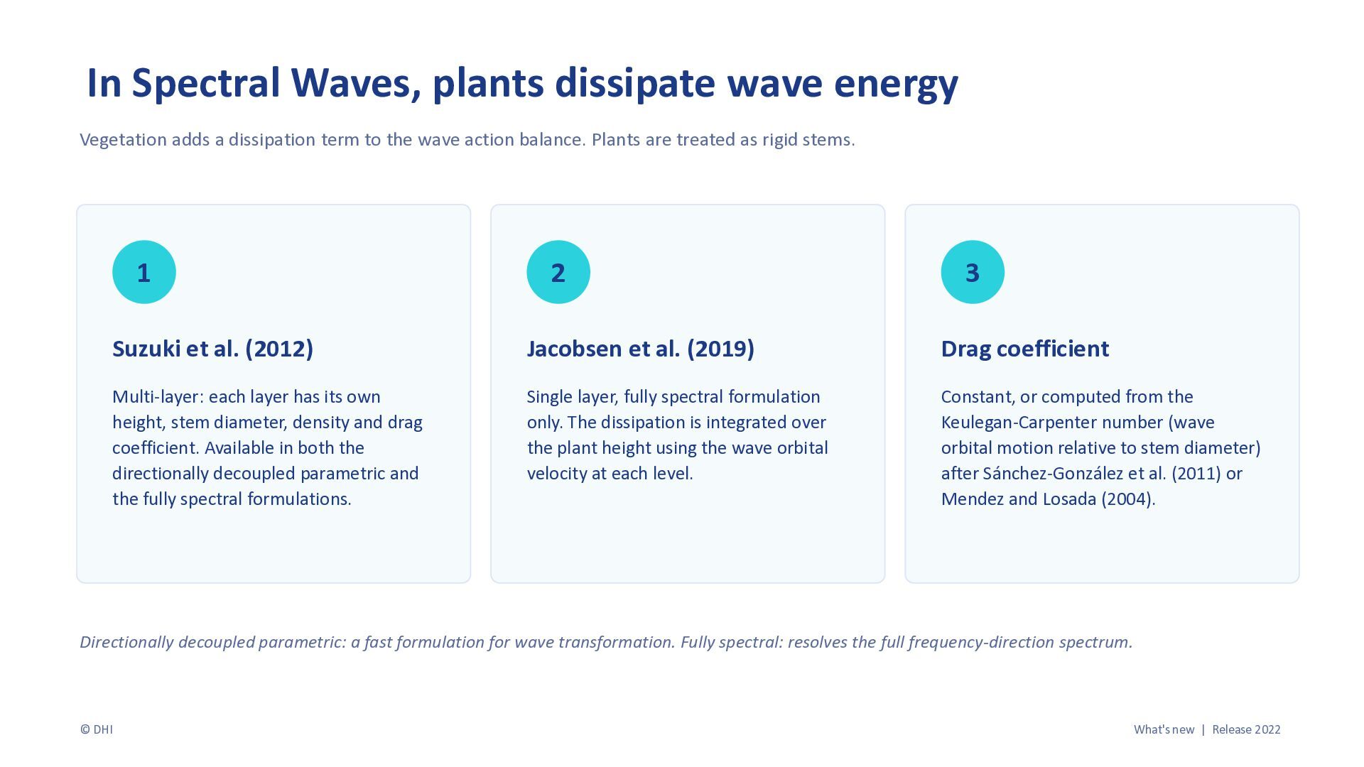
5. In Spectral Waves, plants dissipate wave energy Vegetation adds a dissipation term to the wave action balance. Plants are treated as rigid stems. 1 2 3 Suzuki et al. (2012) Jacobsen et al. (2019) Drag coefficient Multi-layer: each layer has its own height, stem diameter, density and drag coefficient. Available in both the directionally decoupled parametric and the fully spectral formulations. Single layer, fully spectral formulation only. The dissipation is integrated over the plant height using the wave orbital velocity at each level. Constant, or computed from the Keulegan-Carpenter number (wave orbital motion relative to stem diameter) after Sánchez-González et al. (2011) or Mendez and Losada (2004). Directionally decoupled parametric: a fast formulation for wave transformation. Fully spectral: resolves the full frequency-direction spectrum. © DHI What's new | Release 2022
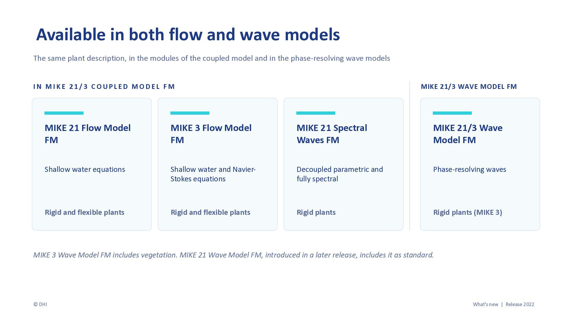
6. Available in both flow and wave models The same plant description, in the modules of the coupled model and in the phase-resolving wave models IN MIKE 21/3 COUPLED MODEL FM MIKE 21/3 WAVE MODEL FM MIKE 21 Flow Model FM MIKE 3 Flow Model FM MIKE 21 Spectral Waves FM MIKE 21/3 Wave Model FM Shallow water equations Shallow water and NavierStokes equations Decoupled parametric and fully spectral Phase-resolving waves Rigid and flexible plants Rigid and flexible plants Rigid plants Rigid plants (MIKE 3) MIKE 3 Wave Model FM includes vegetation. MIKE 21 Wave Model FM, introduced in a later release, includes it as standard. © DHI What's new | Release 2022
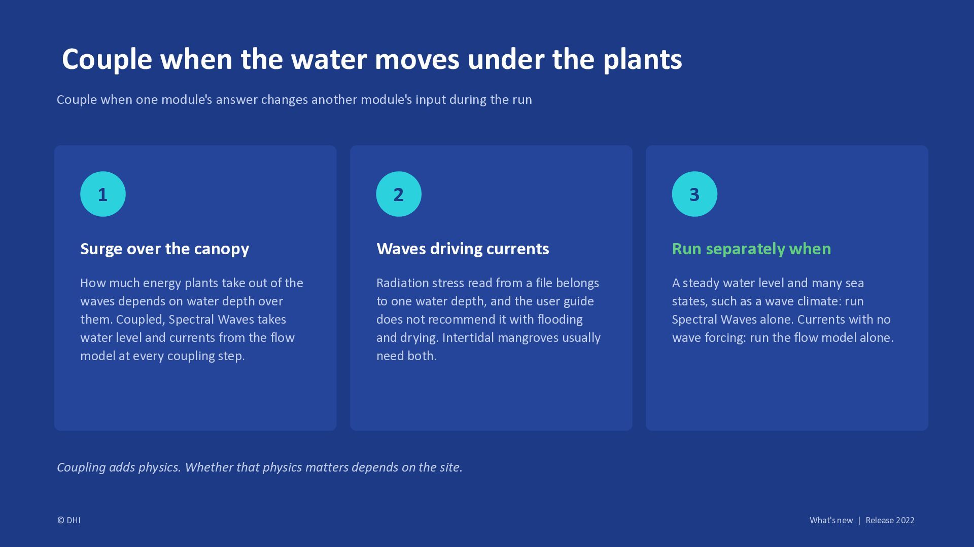
7. Couple when the water moves under the plants Couple when one module's answer changes another module's input during the run 1 2 3 Surge over the canopy Waves driving currents Run separately when How much energy plants take out of the waves depends on water depth over them. Coupled, Spectral Waves takes water level and currents from the flow model at every coupling step. Radiation stress read from a file belongs to one water depth, and the user guide does not recommend it with flooding and drying. Intertidal mangroves usually need both. A steady water level and many sea states, such as a wave climate: run Spectral Waves alone. Currents with no wave forcing: run the flow model alone. Coupling adds physics. Whether that physics matters depends on the site. © DHI What's new | Release 2022
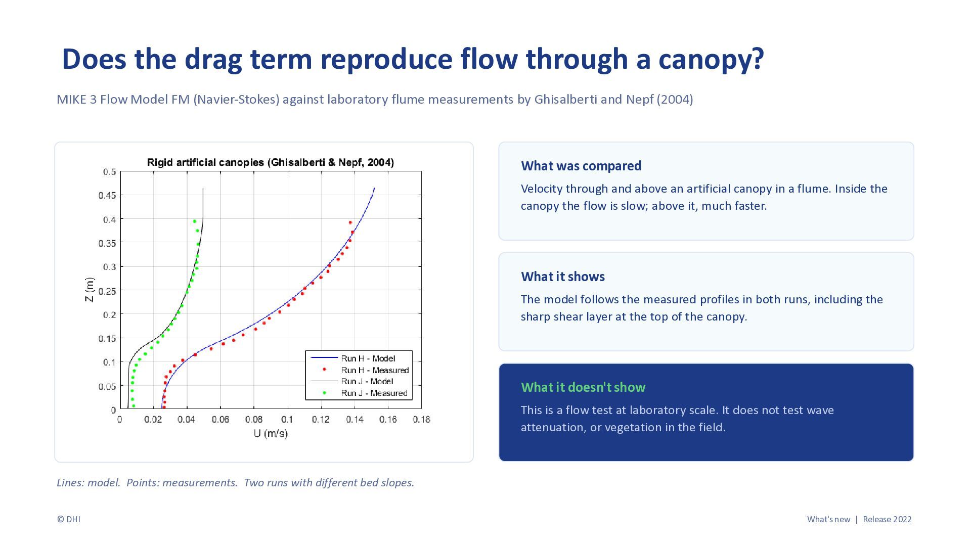
8. Does the drag term reproduce flow through a canopy? MIKE 3 Flow Model FM (Navier-Stokes) against laboratory flume measurements by Ghisalberti and Nepf (2004) What was compared Velocity through and above an artificial canopy in a flume. Inside the canopy the flow is slow; above it, much faster. What it shows The model follows the measured profiles in both runs, including the sharp shear layer at the top of the canopy. What it doesn't show This is a flow test at laboratory scale. It does not test wave attenuation, or vegetation in the field. Lines: model. Points: measurements. Two runs with different bed slopes. © DHI What's new | Release 2022
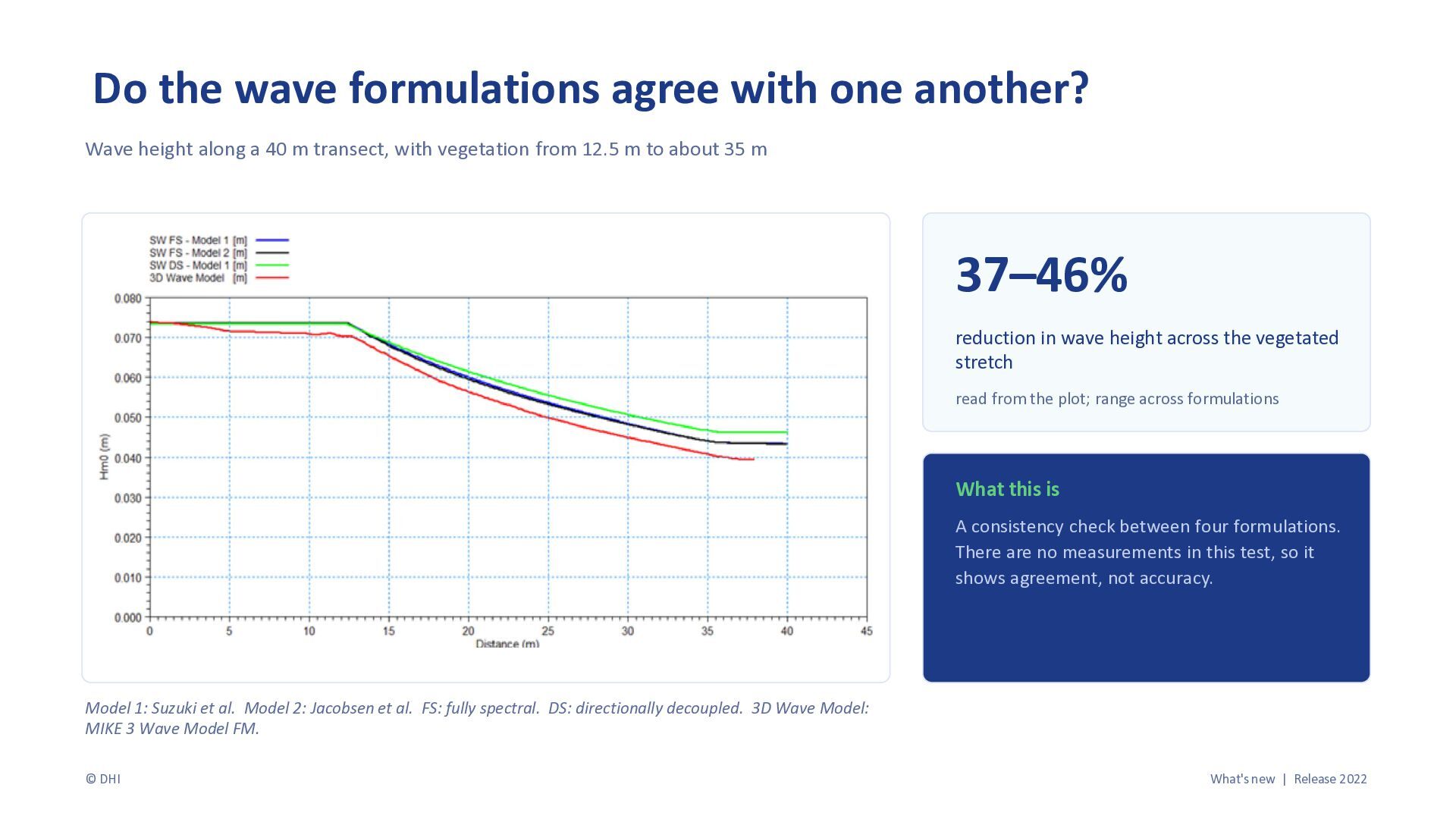
9. Do the wave formulations agree with one another? Wave height along a 40 m transect, with vegetation from 12.5 m to about 35 m 37–46% reduction in wave height across the vegetated stretch read from the plot; range across formulations What this is A consistency check between four formulations. There are no measurements in this test, so it shows agreement, not accuracy. Model 1: Suzuki et al. Model 2: Jacobsen et al. FS: fully spectral. DS: directionally decoupled. 3D Wave Model: MIKE 3 Wave Model FM. © DHI What's new | Release 2022
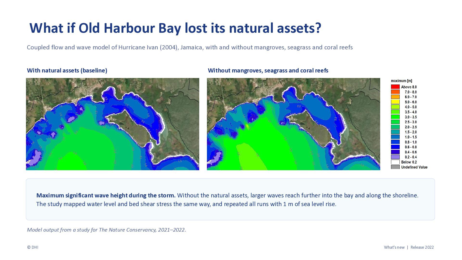
10. What if Old Harbour Bay lost its natural assets? Coupled flow and wave model of Hurricane Ivan (2004), Jamaica, with and without mangroves, seagrass and coral reefs With natural assets (baseline) Without mangroves, seagrass and coral reefs Maximum significant wave height during the storm. Without the natural assets, larger waves reach further into the bay and along the shoreline. The study mapped water level and bed shear stress the same way, and repeated all runs with 1 m of sea level rise. Model output from a study for The Nature Conservancy, 2021–2022. © DHI What's new | Release 2022
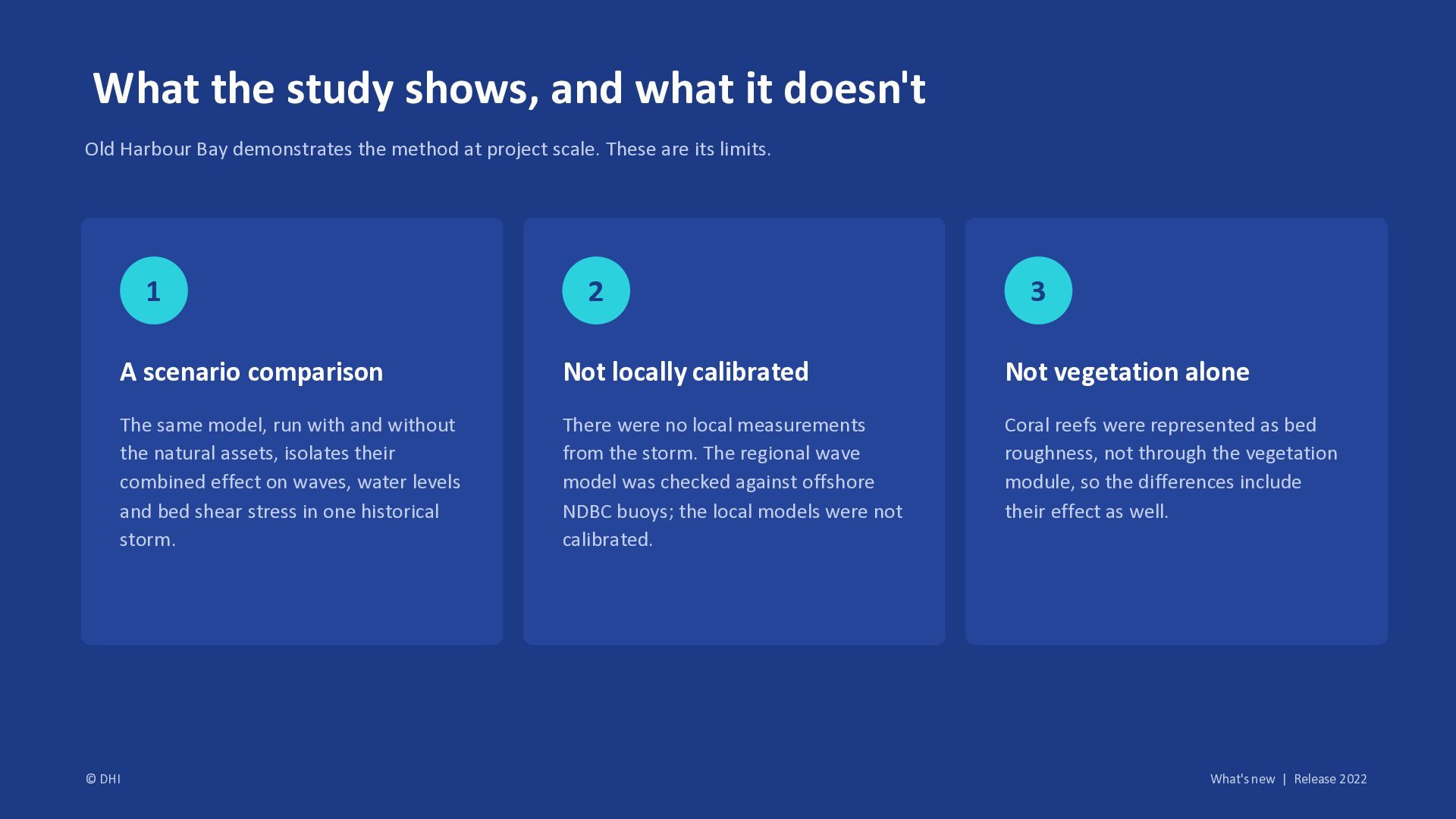
11. What the study shows, and what it doesn't Old Harbour Bay demonstrates the method at project scale. These are its limits. 1 © DHI 2 3 A scenario comparison Not locally calibrated Not vegetation alone The same model, run with and without the natural assets, isolates their combined effect on waves, water levels and bed shear stress in one historical storm. There were no local measurements from the storm. The regional wave model was checked against offshore NDBC buoys; the local models were not calibrated. Coral reefs were represented as bed roughness, not through the vegetation module, so the differences include their effect as well. What's new | Release 2022
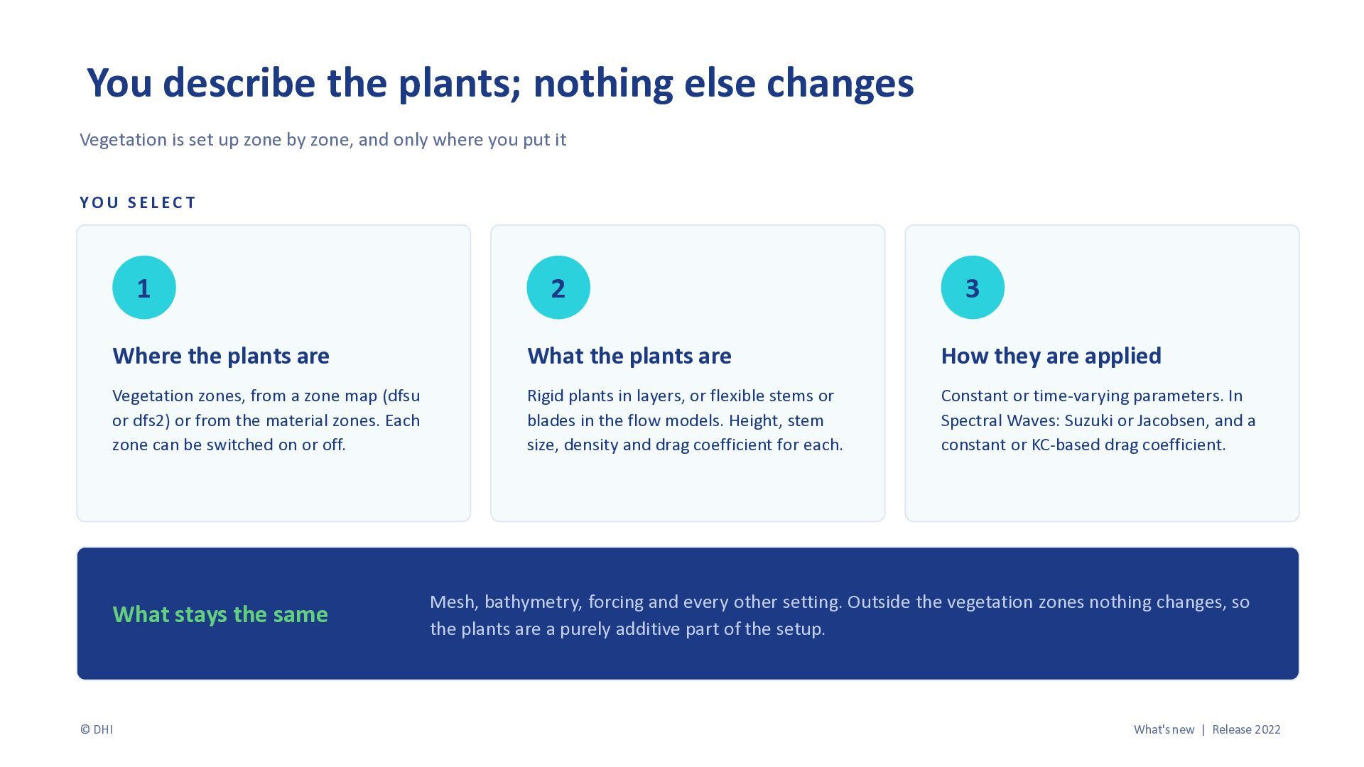
12. You describe the plants; nothing else changes Vegetation is set up zone by zone, and only where you put it YOU SELECT 1 3 Where the plants are What the plants are How they are applied Vegetation zones, from a zone map (dfsu or dfs2) or from the material zones. Each zone can be switched on or off. Rigid plants in layers, or flexible stems or blades in the flow models. Height, stem size, density and drag coefficient for each. Constant or time-varying parameters. In Spectral Waves: Suzuki or Jacobsen, and a constant or KC-based drag coefficient. What stays the same © DHI 2 Mesh, bathymetry, forcing and every other setting. Outside the vegetation zones nothing changes, so the plants are a purely additive part of the setup. What's new | Release 2022
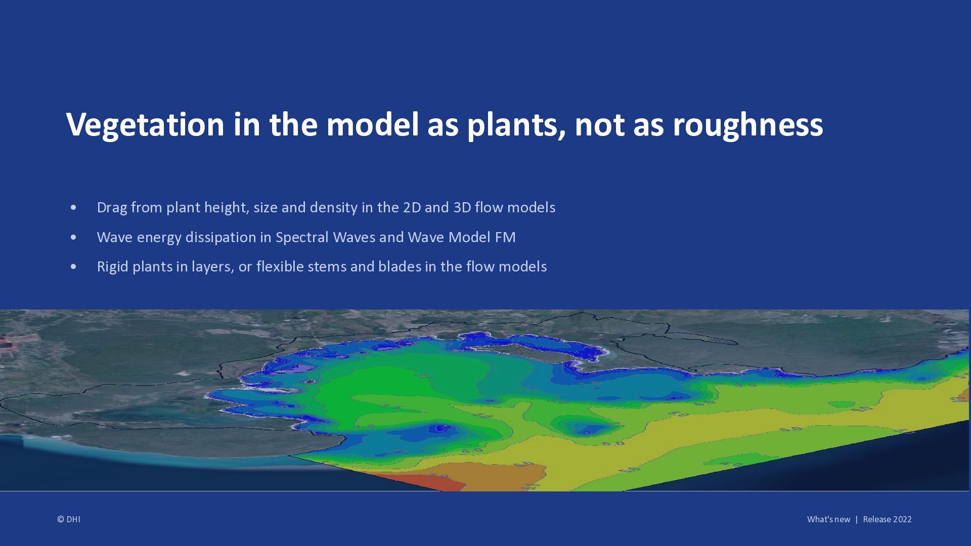
13. Vegetation in the model as plants, not as roughness • Drag from plant height, size and density in the 2D and 3D flow models • Wave energy dissipation in Spectral Waves and Wave Model FM • Rigid plants in layers, or flexible stems and blades in the flow models © DHI What's new | Release 2022