Submesh: fine-mesh answers at coarse-mesh speed

MIKE 21 Flow Model FM solves on a coarse mesh while resolving bathymetry, water depth and roughness on a finer sub-grid. In a Buffalo, New York urban flood model, it used 31× fewer cells with 7.8× more terrain detail. Peak water depths agreed closely with a classic fine-mesh reference. Release 2027.

Transcript

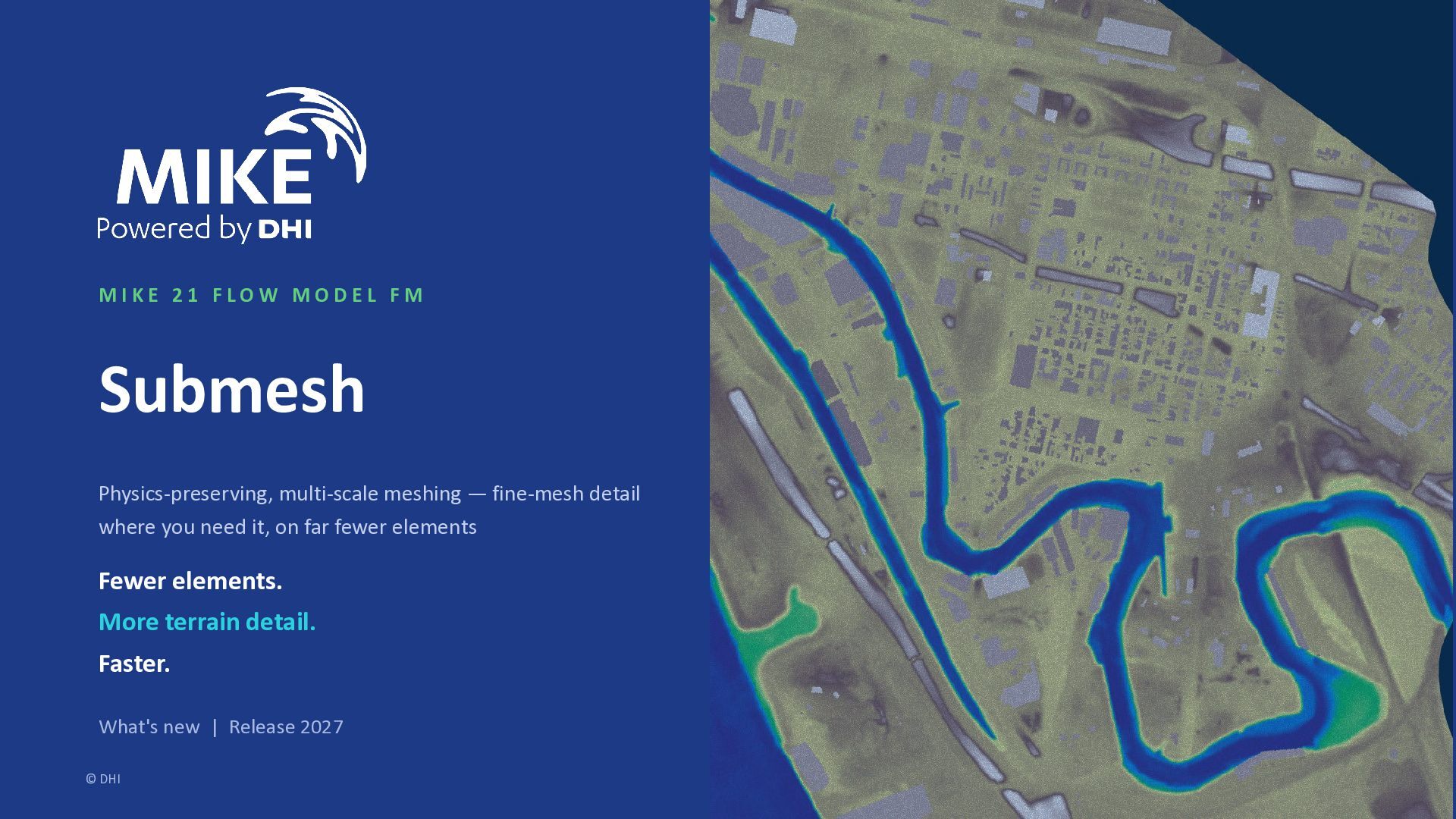
1. MIKE 21 FLOW MODEL FM Submesh Physics-preserving, multi-scale meshing — fine-mesh detail where you need it, on far fewer elements Fewer elements. More terrain detail. Faster. What's new | Release 2027 © DHI
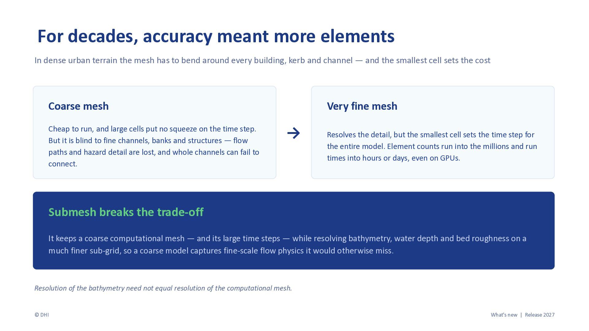
2. For decades, accuracy meant more elements In dense urban terrain the mesh has to bend around every building, kerb and channel — and the smallest cell sets the cost Coarse mesh Cheap to run, and large cells put no squeeze on the time step. But it is blind to fine channels, banks and structures — flow paths and hazard detail are lost, and whole channels can fail to connect. Very fine mesh → Resolves the detail, but the smallest cell sets the time step for the entire model. Element counts run into the millions and run times into hours or days, even on GPUs. Submesh breaks the trade-off It keeps a coarse computational mesh — and its large time steps — while resolving bathymetry, water depth and bed roughness on a much finer sub-grid, so a coarse model captures fine-scale flow physics it would otherwise miss. Resolution of the bathymetry need not equal resolution of the computational mesh. © DHI What's new | Release 2027
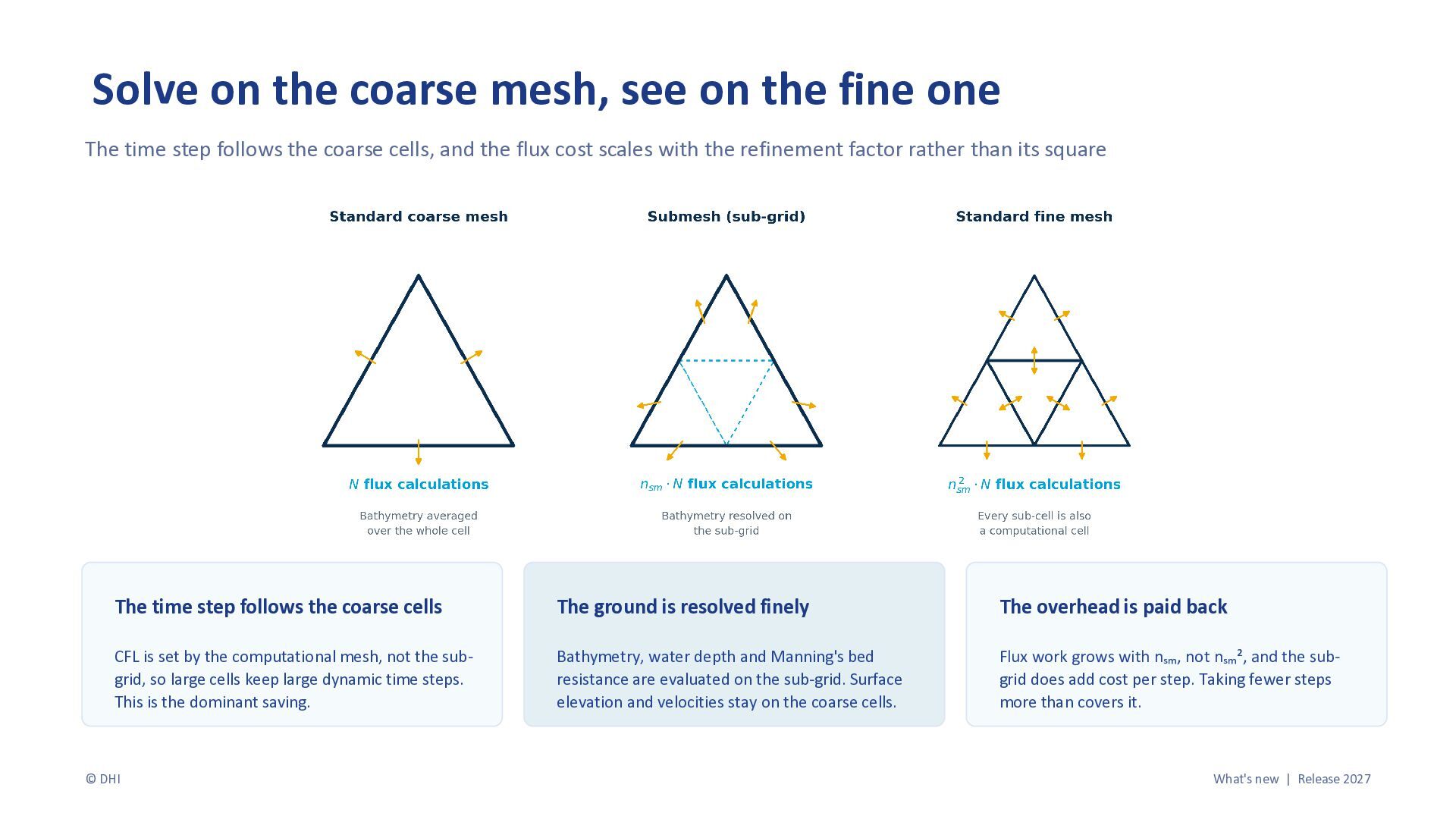
3. Solve on the coarse mesh, see on the fine one The time step follows the coarse cells, and the flux cost scales with the refinement factor rather than its square The time step follows the coarse cells The ground is resolved finely The overhead is paid back CFL is set by the computational mesh, not the subgrid, so large cells keep large dynamic time steps. This is the dominant saving. Bathymetry, water depth and Manning's bed resistance are evaluated on the sub-grid. Surface elevation and velocities stay on the coarse cells. Flux work grows with nₛₘ, not nₛₘ², and the subgrid does add cost per step. Taking fewer steps more than covers it. © DHI What's new | Release 2027
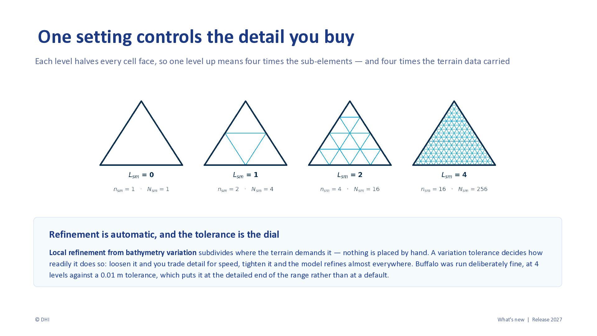
4. One setting controls the detail you buy Each level halves every cell face, so one level up means four times the sub-elements — and four times the terrain data carried Refinement is automatic, and the tolerance is the dial Local refinement from bathymetry variation subdivides where the terrain demands it — nothing is placed by hand. A variation tolerance decides how readily it does so: loosen it and you trade detail for speed, tighten it and the model refines almost everywhere. Buffalo was run deliberately fine, at 4 levels against a 0.01 m tolerance, which puts it at the detailed end of the range rather than at a default. © DHI What's new | Release 2027
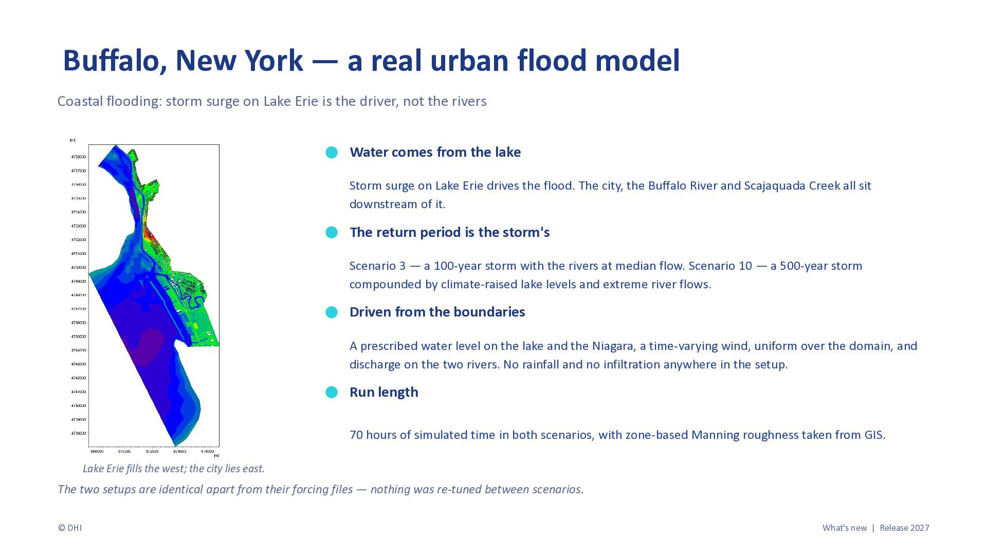
5. Buffalo, New York — a real urban flood model Coastal flooding: storm surge on Lake Erie is the driver, not the rivers Water comes from the lake Storm surge on Lake Erie drives the flood. The city, the Buffalo River and Scajaquada Creek all sit downstream of it. The return period is the storm's Scenario 3 — a 100-year storm with the rivers at median flow. Scenario 10 — a 500-year storm compounded by climate-raised lake levels and extreme river flows. Driven from the boundaries A prescribed water level on the lake and the Niagara, a time-varying wind, uniform over the domain, and discharge on the two rivers. No rainfall and no infiltration anywhere in the setup. Run length 70 hours of simulated time in both scenarios, with zone-based Manning roughness taken from GIS. Lake Erie fills the west; the city lies east. The two setups are identical apart from their forcing files — nothing was re-tuned between scenarios. © DHI What's new | Release 2027
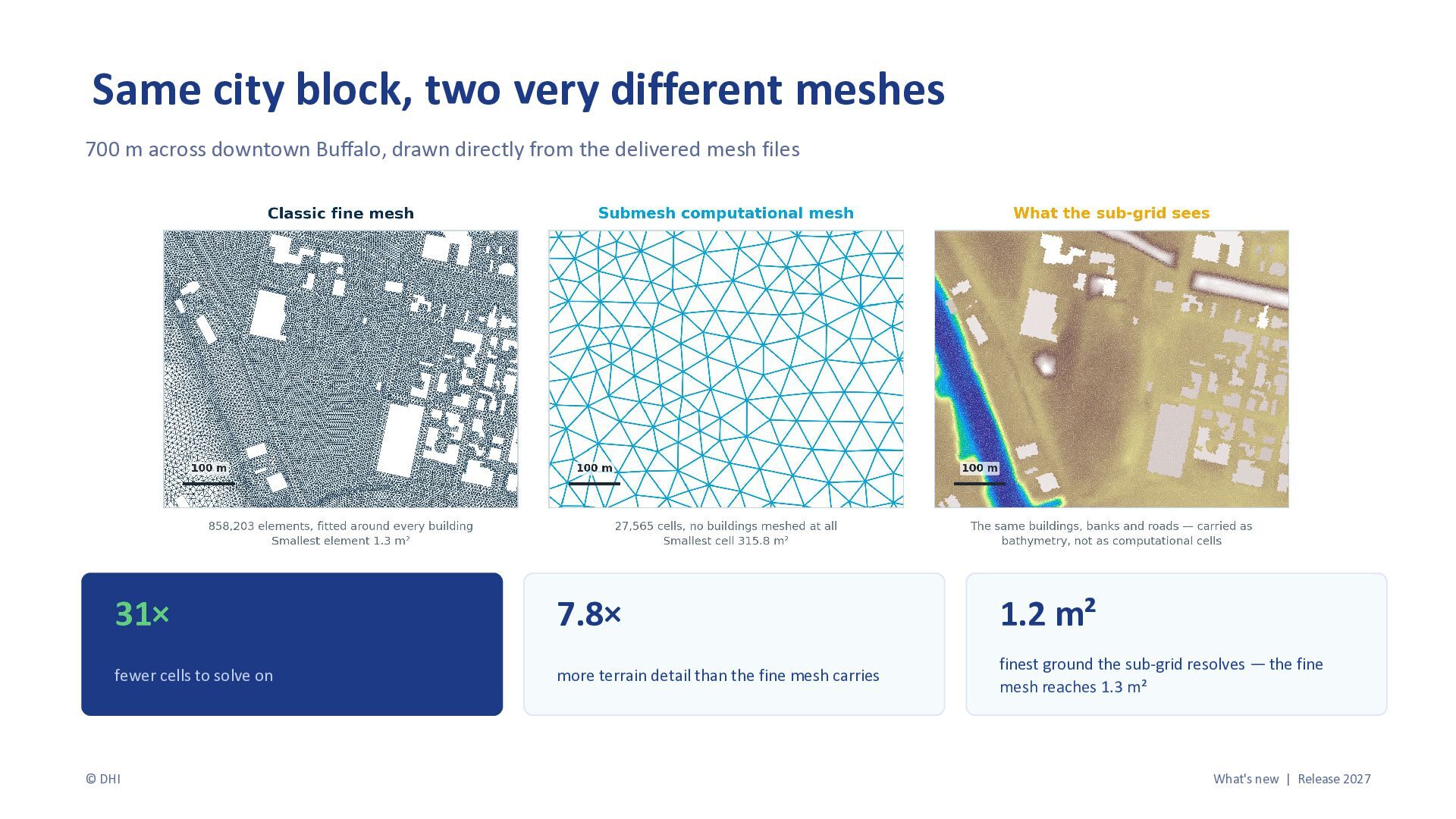
6. Same city block, two very different meshes 700 m across downtown Buffalo, drawn directly from the delivered mesh files 31× 7.8× 1.2 m² fewer cells to solve on more terrain detail than the fine mesh carries finest ground the sub-grid resolves — the fine mesh reaches 1.3 m² © DHI What's new | Release 2027
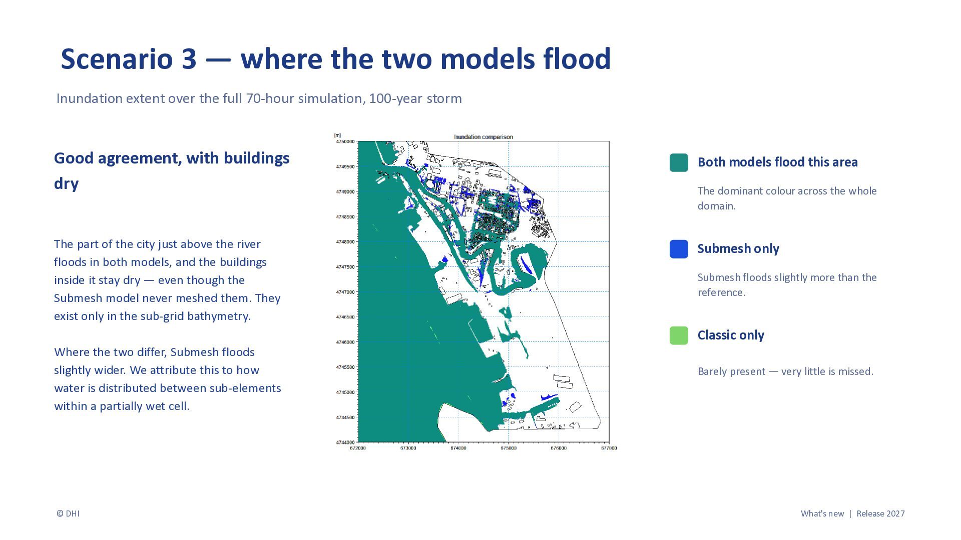
7. Scenario 3 — where the two models flood Inundation extent over the full 70-hour simulation, 100-year storm Good agreement, with buildings dry The part of the city just above the river floods in both models, and the buildings inside it stay dry — even though the Submesh model never meshed them. They exist only in the sub-grid bathymetry. Where the two differ, Submesh floods slightly wider. We attribute this to how water is distributed between sub-elements within a partially wet cell. © DHI Both models flood this area The dominant colour across the whole domain. Submesh only Submesh floods slightly more than the reference. Classic only Barely present — very little is missed. What's new | Release 2027
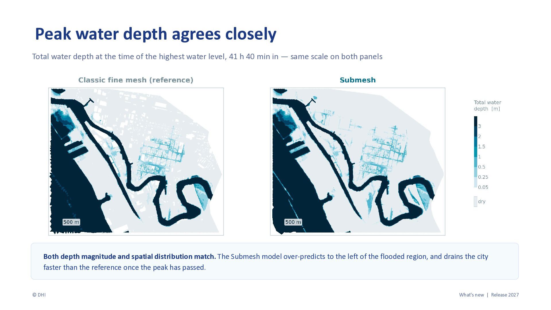
8. Peak water depth agrees closely Total water depth at the time of the highest water level, 41 h 40 min in — same scale on both panels Both depth magnitude and spatial distribution match. The Submesh model over-predicts to the left of the flooded region, and drains the city faster than the reference once the peak has passed. © DHI What's new | Release 2027
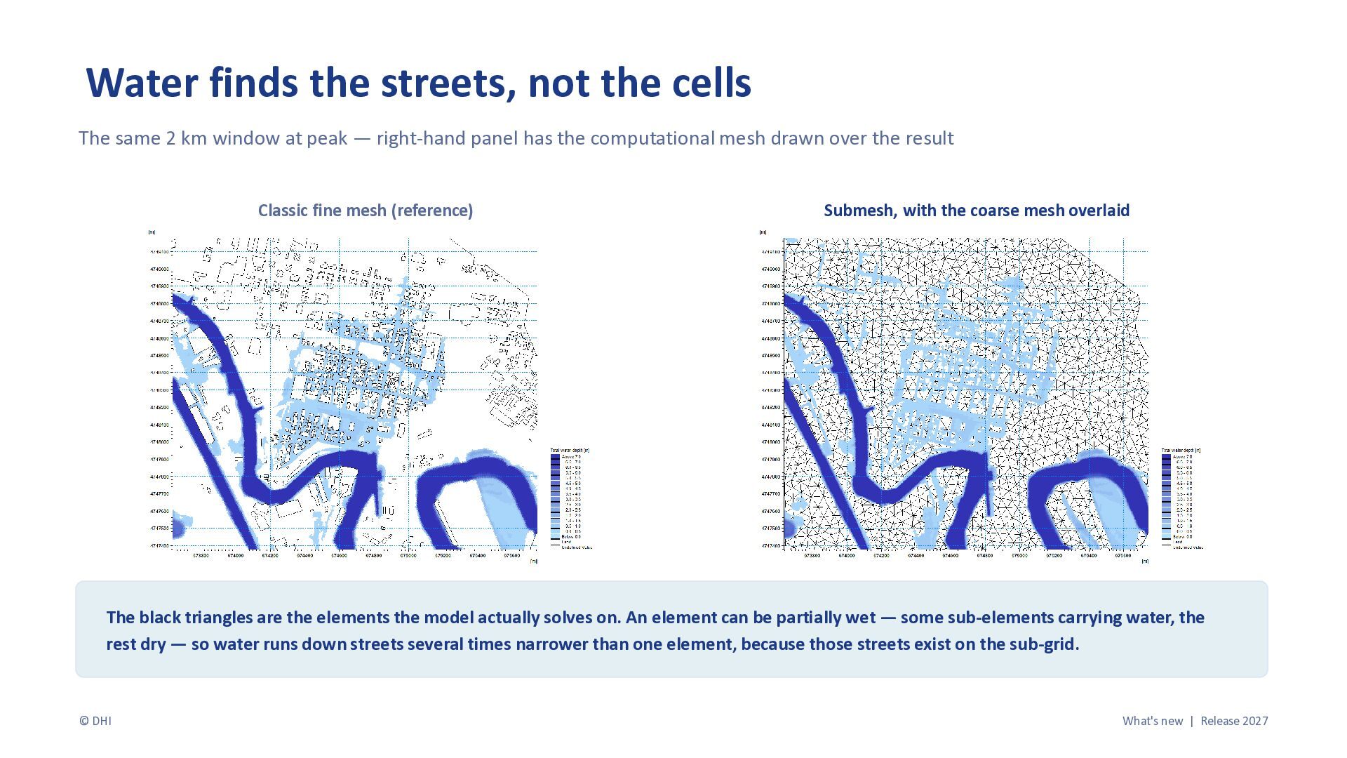
9. Water finds the streets, not the cells The same 2 km window at peak — right-hand panel has the computational mesh drawn over the result Classic fine mesh (reference) Submesh, with the coarse mesh overlaid The black triangles are the elements the model actually solves on. An element can be partially wet — some sub-elements carrying water, the rest dry — so water runs down streets several times narrower than one element, because those streets exist on the sub-grid. © DHI What's new | Release 2027
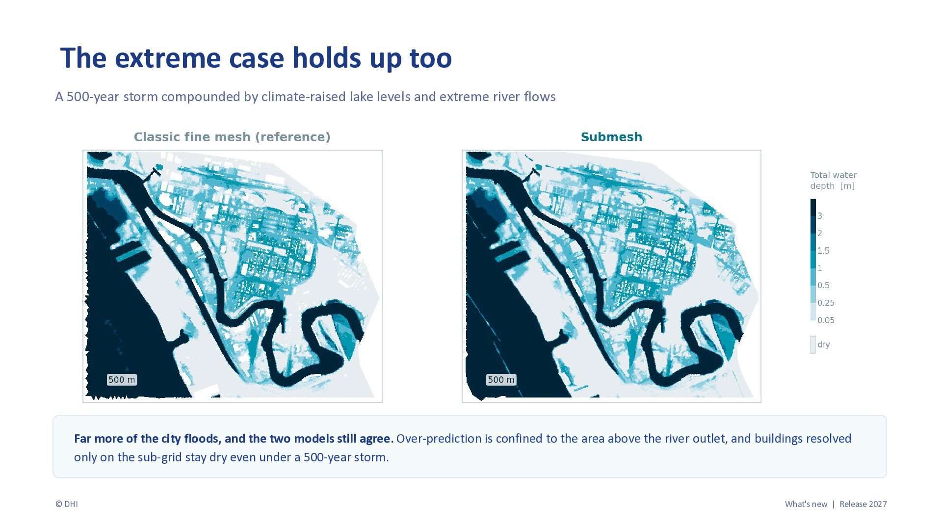
10. The extreme case holds up too A 500-year storm compounded by climate-raised lake levels and extreme river flows Far more of the city floods, and the two models still agree. Over-prediction is confined to the area above the river outlet, and buildings resolved only on the sub-grid stay dry even under a 500-year storm. © DHI What's new | Release 2027
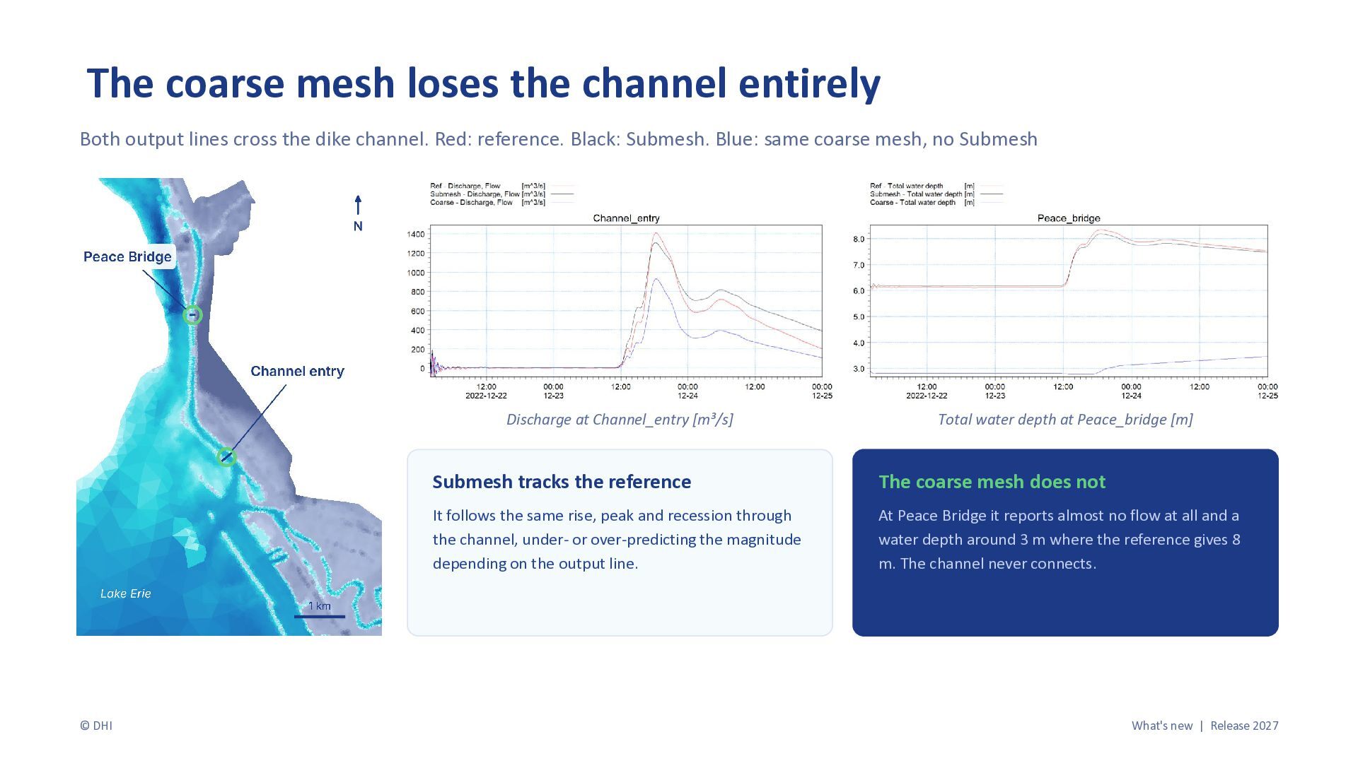
11. The coarse mesh loses the channel entirely Both output lines cross the dike channel. Red: reference. Black: Submesh. Blue: same coarse mesh, no Submesh Discharge at Channel_entry [m³/s] © DHI Total water depth at Peace_bridge [m] Submesh tracks the reference The coarse mesh does not It follows the same rise, peak and recession through the channel, under- or over-predicting the magnitude depending on the output line. At Peace Bridge it reports almost no flow at all and a water depth around 3 m where the reference gives 8 m. The channel never connects. What's new | Release 2027
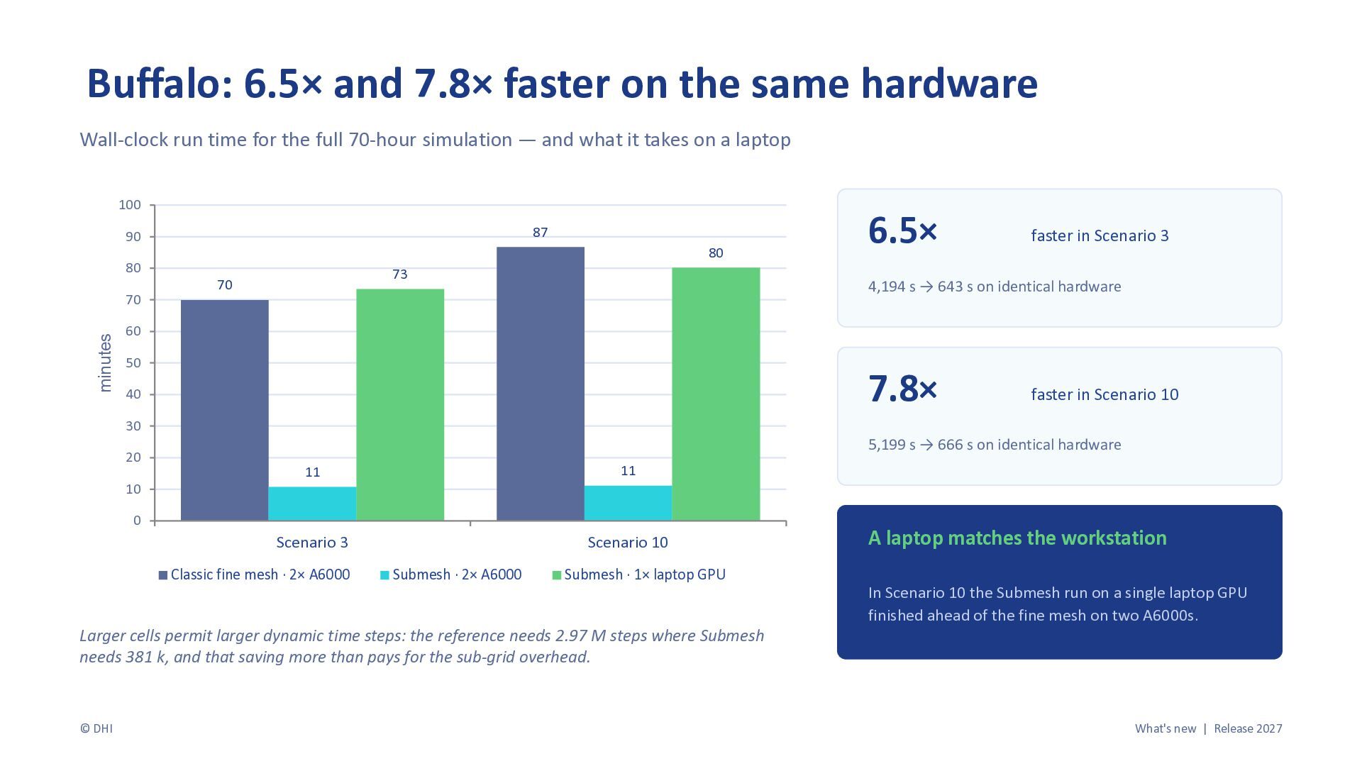
12. Buffalo: 6.5× and 7.8× faster on the same hardware Wall-clock run time for the full 70-hour simulation — and what it takes on a laptop 100 87 90 80 minutes 70 80 73 70 faster in Scenario 3 4,194 s → 643 s on identical hardware 60 50 7.8× 40 30 20 10 faster in Scenario 10 5,199 s → 666 s on identical hardware 11 11 Scenario 3 Scenario 10 0 Classic fine mesh · 2× A6000 Submesh · 2× A6000 Submesh · 1× laptop GPU Larger cells permit larger dynamic time steps: the reference needs 2.97 M steps where Submesh needs 381 k, and that saving more than pays for the sub-grid overhead. © DHI 6.5× A laptop matches the workstation In Scenario 10 the Submesh run on a single laptop GPU finished ahead of the fine mesh on two A6000s. What's new | Release 2027
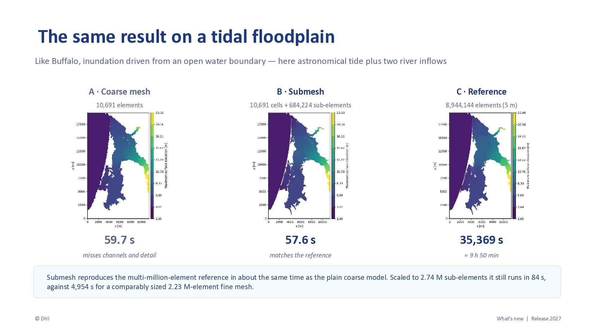
13. The same result on a tidal floodplain Like Buffalo, inundation driven from an open water boundary — here astronomical tide plus two river inflows A · Coarse mesh B · Submesh C · Reference 10,691 elements 10,691 cells + 684,224 sub-elements 8,944,144 elements (5 m) 59.7 s 57.6 s 35,369 s misses channels and detail matches the reference ≈ 9 h 50 min Submesh reproduces the multi-million-element reference in about the same time as the plain coarse model. Scaled to 2.74 M sub-elements it still runs in 84 s, against 4,954 s for a comparably sized 2.23 M-element fine mesh. © DHI What's new | Release 2027
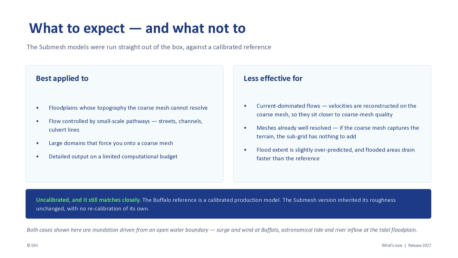
14. What to expect — and what not to The Submesh models were run straight out of the box, against a calibrated reference Best applied to Less effective for • Floodplains whose topography the coarse mesh cannot resolve • • Flow controlled by small-scale pathways — streets, channels, culvert lines Current-dominated flows — velocities are reconstructed on the coarse mesh, so they sit closer to coarse-mesh quality • • Large domains that force you onto a coarse mesh Meshes already well resolved — if the coarse mesh captures the terrain, the sub-grid has nothing to add • Detailed output on a limited computational budget • Flood extent is slightly over-predicted, and flooded areas drain faster than the reference Uncalibrated, and it still matches closely. The Buffalo reference is a calibrated production model. The Submesh version inherited its roughness unchanged, with no re-calibration of its own. Both cases shown here are inundation driven from an open water boundary — surge and wind at Buffalo, astronomical tide and river inflow at the tidal floodplain. © DHI What's new | Release 2027
15. Can a coarse mesh think like a fine mesh? Closely, on our Buffalo case — by using as much of your data as possible, without paying the full computational price. "I need results fast." "I need to use all my data." "My hardware is limited." Coastal and floodplain screening with far greater confidence in flood extents than a coarse mesh can give. Exploit high-resolution survey and LiDAR to the full without a million-element mesh. Build large-domain models that would otherwise be out of reach — including on a laptop. ✓ Full FM numerics — Riemann solver, well-balanced, mass-conserving ✓ Fully implicit friction for stability on steep slopes ✓ FM features retained — structures, sources and infrastructure ✓ Manning's bed resistance computed on the Submesh MIKE 21 Flow Model FM | Submesh | Release 2027 Developed by Max Bitsch as an industrial PhD with DTU Compute and DHI, supervised by Allan Peter Engsig-Karup (DTU), Jesper Grooss and Ole Rene Sørensen (DHI), building on the subgrid method of Casulli (2009) and Sanders et al. (2019). © DHI What's new | Release 2027