SERDP model comparison

A brief overview of metrics of model (forecast) comparison

Transcript

1.   1   A  short  overview  of  model  selection,  validation,   comparison  methodologies  and  metrics  for   seasonal  MLOS  forecasting     Nicolas  Fauchereau   Nicolas.Fauchereau@niwa.co.nz     Introduction       We  need  to  be  able  to  compare  the  performance  of  the  various  (statistical)   models  developed  to  forecast  seasonal  MLOS  anomalies       In  this  short  document,  I  provide  an  overview,  first  of  some  general   consideration  on  this  topic,  then  give  some  more  details  on  the  metrics         Different  types  of  models       There’s  2  main  types  of  models  that  are  /  will  be  developed  as  part  of  the  effort:       1. Regression  models:       In  regression,  we  are  predicting  MLOS  as  a  continuous,  real-­‐valued  variable.       2. Classification  models:       In  this  case,  a  discrete,  qualitative  ‘label’  is  predicted,  in  the  case  of  MLOS,  it  has   been   decided   during   the   November   SERDP   workshop   that   the   –   originally   continuous  -­‐    time-­‐series  of  MLOS  anomalies  will  discretized  nto  5  equi-­‐probable   categories,   based   on   the   empirical   quintiles   calculated   over   the   climatological   period.       Some  clarification  on  the  vocabulary         First   of   all,   I   will   use   ‘the   model’   and   ‘the   forecasts’   interchangeably   from   the   section,  in  the  context  of  this  document  when  I  use  ‘the  model”  I  really  mean  ‘the   set  of  forecasts  generated  by  the  model’.    
2.   2   The   literature   is   somewhat   confusing   about   the   meanings   of   model   selection,   comparison,   validation,   verification,   etc   ….   Below   I’m   providing   some   definitions  so  that  we  all  know  what  we’re  talking  about  in  different  contexts  :       I   will   also   briefly   recall   some   consideration   about   the   model   fitting   process   (learning)  and  why  cross-­‐validation  is  important.       Model  selection       In  this  document,  I’m  referring  to  model  selection  as  the  process  by  which,  for   one  particular  model,  the  best  set  of  hyper-­‐parameters  is  selected.       To  be  clear,  a  ‘hyper-­‐parameter’  is  a  parameter  of  the  model  that  is  basically   manually  set  –  up,  as  opposed  to  the  model’s  parameters  themselves,  which  are   optimized  during  the  learning  (model  fitting)  stage.       Examples  of  parameters,  for  e.g.  a  linear  regression  model,  are  the  alpha  and   beta  parameters  of  the  equation.       An  example  of  hyper-­‐parameter  are  the  “C”  for  Support  Vector  Machines,  or  the   regularization  settings  in  e.g.  ridge  regression.       Model  validation     I’m  referring  to  model   (or   forecast)   validation  as  synonymous  to  model   or   forecast  verification,  forecast  evaluation       Now  we  have  fixed  both  the  parameters  and  the  hyperparameters  of  the  model,   and  we  want  to  evaluate  its  performance.  A  reasonable  thing  to  do  then  is  to   work  in  hindcast  mode,  using  ALL  the  available  pairs  of  forecasts  /  observations,   and  update  these  metrics  on  a  regular  basis,  in  order  to  detect  potential  trends  in   the  forecast  verification  scores       Now  we  can  go  on  exactly  how  the  model’s  forecasts  are  evaluated  compared  to   the   observations,   again   it   will   be   different   between   regression   models   and   classification  models,  but  first  we  need  to  acknowledge  there  are  many  attributes   of  model  performance:       • Accuracy:  average  correspondence  between       • Bias  (systematic):  basically  the  difference  between  the  average  forecast   and  the  average  observed  predictand’s  value.    
3.   3   • Reliability  (or  conditional  bias):  relationship  between  the  forecast  and   the  observed  predictand’s  values  for  specific  values  of  (i.e.  conditional  on)   the  forecast.     • Resolution:   Pertains   to   the   differences   between   the   conditional   averages   of   the   observations   for   different   values   of   the   forecast:   if   this   difference  is  low,  the  forecast  (the  model)  has  poor  resolution,  if  it  is  high,   the   forecast   has   good   resolution.   It   refers   to   the   degree   to   which   the   model  sort  the  observed  values  into  groups  that  are  different  from  each   other.       • Discrimination:   is   the   converse   of   resolution,   it   pertains   to   the   differences  between  the  conditional  averages  of  the  forecasts  for  different   values  of  the  observations.       • Sharpness:  is  related  to  the  characteristic  of  the  forecasts  alone  (without   reference   to   the   observations)   in   terms   of   their   unconditional   distribution:  in  short,  forecasts  that  rarely  deviate  from  the  climatology   are  not  sharp,  while  those  who  do  are  …     All   these   attributes   can   usually   be   summed   up   in   scalar   values   for   either   continuous  or  categorical  forecasts,  and  these  scalar  measures  can  be  combined   into  skill  scores  (see  below).     Forecast  skill       What  we  really  want  is  a  measure  of  the  forecasts  SKILL,  i.e.  a  measure  of  the   accuracy  (see  above)  of  the  set  of  forecasts  relative  to  ‘control’  forecasts.   There  are  a  few  options  for  generating  the  ‘control’  forecasts,  the  most  common   being:       • Using  persistence     • Using  climatology     • Using   random   forecasts   based   on   the   observations   fitted   to   a   distribution.       The  skill  scores  are  usually  scaled  so  that  they  reach  1  for  a  ‘perfect’  forecast,  0   when  the  forecasts  are  no  better  than  the  reference  forecast,  and  take  negative   values  when  it  performs  worse  than  the  reference  forecast.     What  skill-­‐scores  to  use:       Regression      
4.   4   For   regression,   the   R-­‐squared   is   usually   used   as   a   metric   during   the   model   selection  phase.  However,  and  for  model  comparison’s  sake,  it  is  better  to  use  a   skill  score  that  uses  penalties  relating  to  the  reliability  and  bias  of  the  forecasts.     • MAE  (Mean  Absolute  Error):       Is  the  average  of  the  absolute  values  of  the  difference  between  the  forecast  and   observation  pairs:     1 ! −  ! ! !!!     • The  MSE  (Mean  Square  Error)     The  MSE  is  the  average  squared  difference  between  the  forecast  and  observation   pairs:         1 ! −  ! ! ! !!!     Often  the  RMSE  is  given,  calculated  as  the  square-­‐root  of  the  MSE.     To  translate  either  MAE  or  MSE  into  a  skill  measure  (see  above)  one  can  then   simply  calculate  the  MAE  or  MSE  of  a  climatology-­‐based  forecast.       This  skill  score,  for  the  MSE,  is  simply:       !"# =  1 −   !"#$       It  can  be  shown  that  this  latter  equation  for  the  MSE  skill  score  is  equivalent  to   the  correlation  coefficient  (Pearson’s  correlation  coefficient)  penalized  for  terms   that   take   into   account   respectively   the   reliability   (term   that   is   0   if   there   is   no   conditional  bias)  and  the  systematic  (unconditional)  bias.     Classification       First  of  all  we’re  going  to  assume  that  all  classification  models  that  we  are  going   to   explore   give   probabilistic   forecasts:   i.e.   a   given   discrete   probability   is   assigned  to  each  category  of  the  predictand,  (and  these  probabilities  sum  to  1  !).      
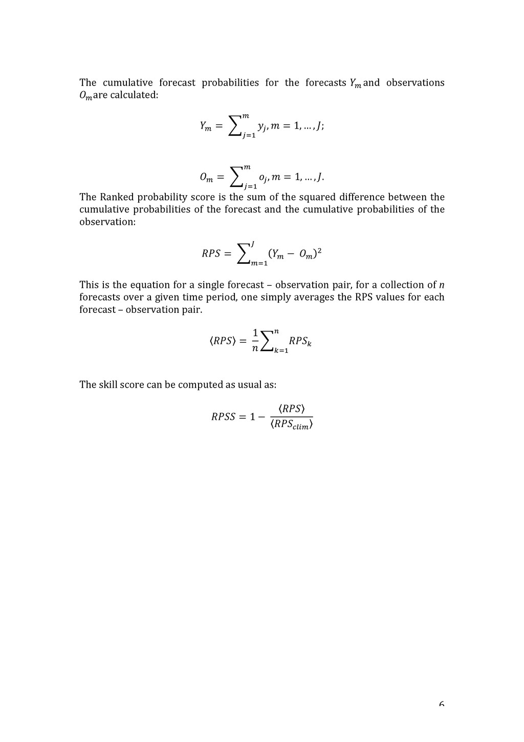
5.   5   We’re   also   going   to   assume   that   the   reference   forecast   is   simply   a   climatological   forecast   (i.e.   in   the   case   of   quintile-­‐based   categories,   equal   probabilities  of  0.2  are  assigned  to  each  category).     Lastly,  we’re  going  to  assume  that  we  are  interested  into  skill  metrics  that  takes   into  account  the  uncertainty   in   the   forecast,  i.e.  they   actually   consider   the   distribution  of  the  discrete  probability  values  assigned  to  each  category.       Lastly   another   constraint   is   that   the   categorical   (quintile   based)   MLOS   predictand   is   ordinal   (i.e.   the   categories   are   naturally   ordered   from   e.g.   ‘well   below  normal’  to  ‘well  above  normal’)  and  thus  the  magnitude  of  the  potential   forecast  error  is  important.     Another   option   (which   will   NOT   be   discussed   here)   is   to   ignore   the   forecast’s   uncertainty,  by  only  considering  the  category  to  which  the  highest  probability  is   assigned  by  the  model.  In  this  case,  skill  scores  based  on  the  calculation  of  hit   rates,  such  as  the  Heidke  Skill  Score  or  Peirce  Skill  Scores  can  be  used:  their   extensive  description  can  be  found  in  the  IRI’s  ‘Descriptions  of  the  IRI  climate   forecast  verification  scores  document,  available  at  URL:       http://iri.columbia.edu/wp-­‐content/uploads/2013/07/scoredescriptions.pdf     Given   all   the   assumptions   and   constraints   above   (probabilistic   forecasts,   reference  forecast  is  climatology,  uncertainty  in  the  forecast  must  be  taken  into   account  for  the  calculation  of  the  skill  score,  predictand  is  an  ordinal  categorical   variable),   the   metric   that   I   recommend   to   compare   the   performance   of   the   classification  models  is  the  Ranked  Probability  Skill  Score  (RPSS).       The  Ranked  Probability  Skill  Score  (RPSS)     As   usual,   the   RPSS   is   based   on   the   scaling   of   one   metric,   namely   the   Ranked   Probability   Score   (RPS)   of   the   actual   forecast   to   the   one   calculated   for   a   reference  forecast  (again  here  climatological  forecast).       The  RPS  is  essentially  an  extension  of  the  Brier  Score  to  multiple  (more  than  2)   category  events.     Let  J  be  the  number  of  categories  (5)  events  and  therefore  also  the  number  of   probabilities  included  in  each  forecast.  The  forecast  vector  is  constituted  of  the   forecast  probabilities,  summing  to  1,  e.g.:  for  a  5  categories  forecast:       Y1  =  0.05,  y2=0.1,  y3=  0.2,  y4=0.25,  y5=0.4     The  observation  vector  has  also  5  components,  with  the  observed  outcome  set  to   1  and  the  other  components  set  to  0,  i.e.  in  the  case  of  observed  MLOS  anomaly   above  the  80th  percentile  (‘well-­‐above’  category)  the  observation  vector  is       Y1  =  0,  y2=0,  y3=  0,  y4=0,  y5=1    
6.   6     The   cumulative   forecast   probabilities   for   the   forecasts  ! and   observations   ! are  calculated:       ! =   ! , = 1, … , ; ! !!!       ! =   ! , = 1, … , . ! !!!   The  Ranked  probability  score  is  the  sum  of  the  squared  difference  between  the   cumulative  probabilities  of  the  forecast  and  the  cumulative  probabilities  of  the   observation:       =   ! −  ! ! ! !!!     This  is  the  equation  for  a  single  forecast  –  observation  pair,  for  a  collection  of  n   forecasts  over  a  given  time  period,  one  simply  averages  the  RPS  values  for  each   forecast  –  observation  pair.       =   1 ! ! !!!         The  skill  score  can  be  computed  as  usual  as:       = 1 −   !"#$