Using novel data to provide local insights

A presentation given to the Royal Statistical Society

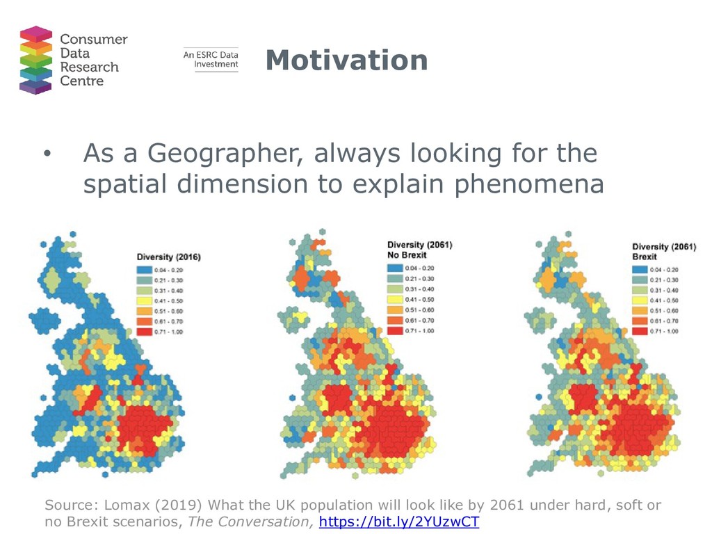
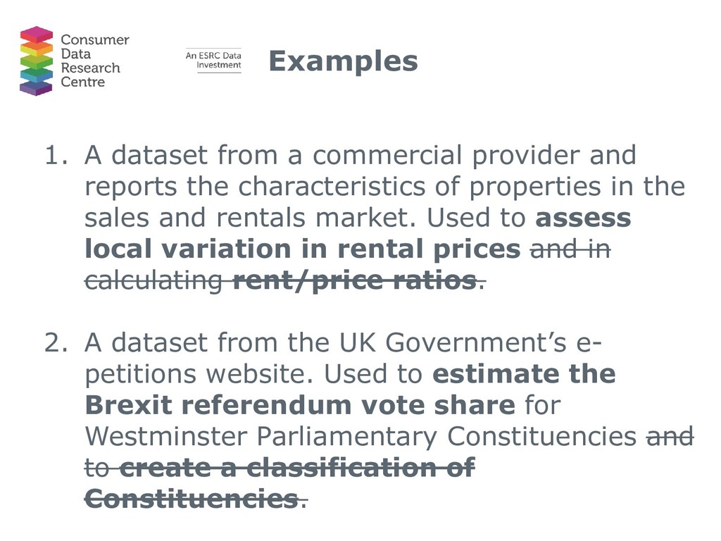
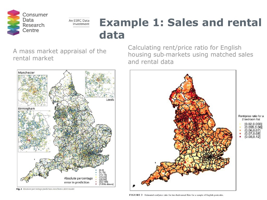
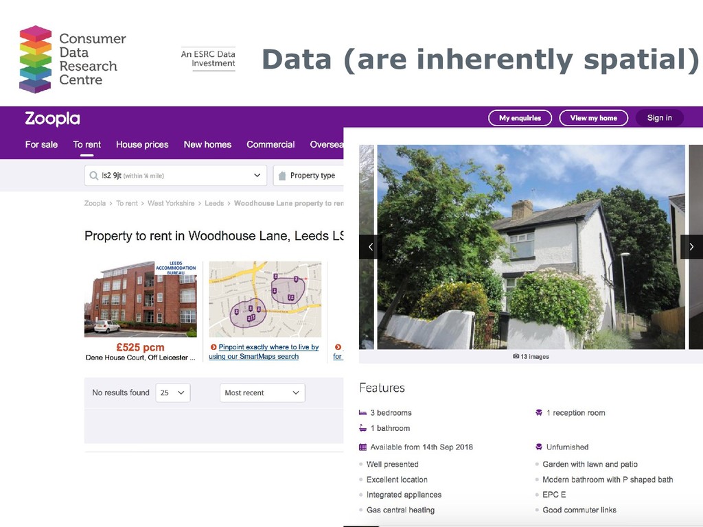
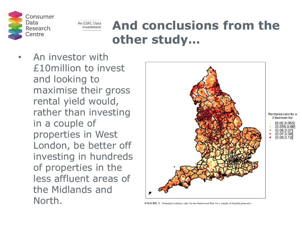
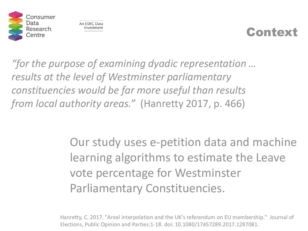
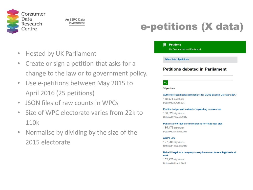
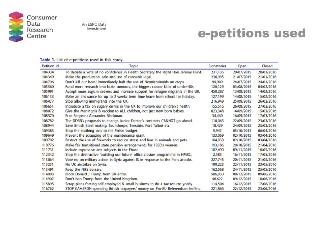
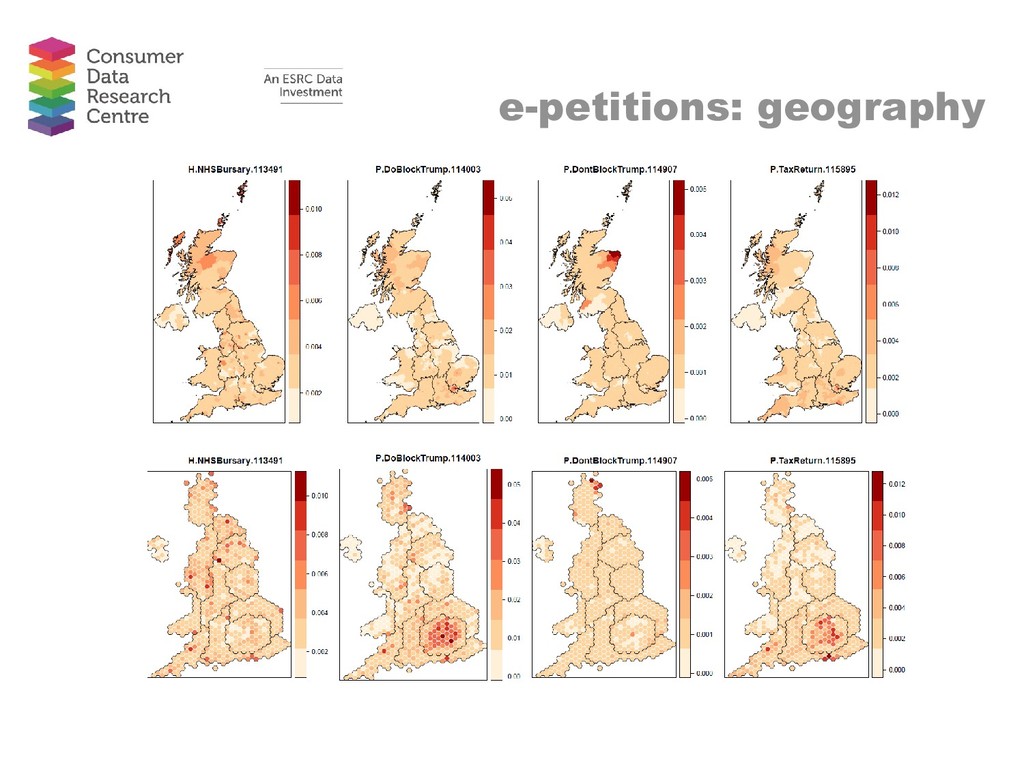
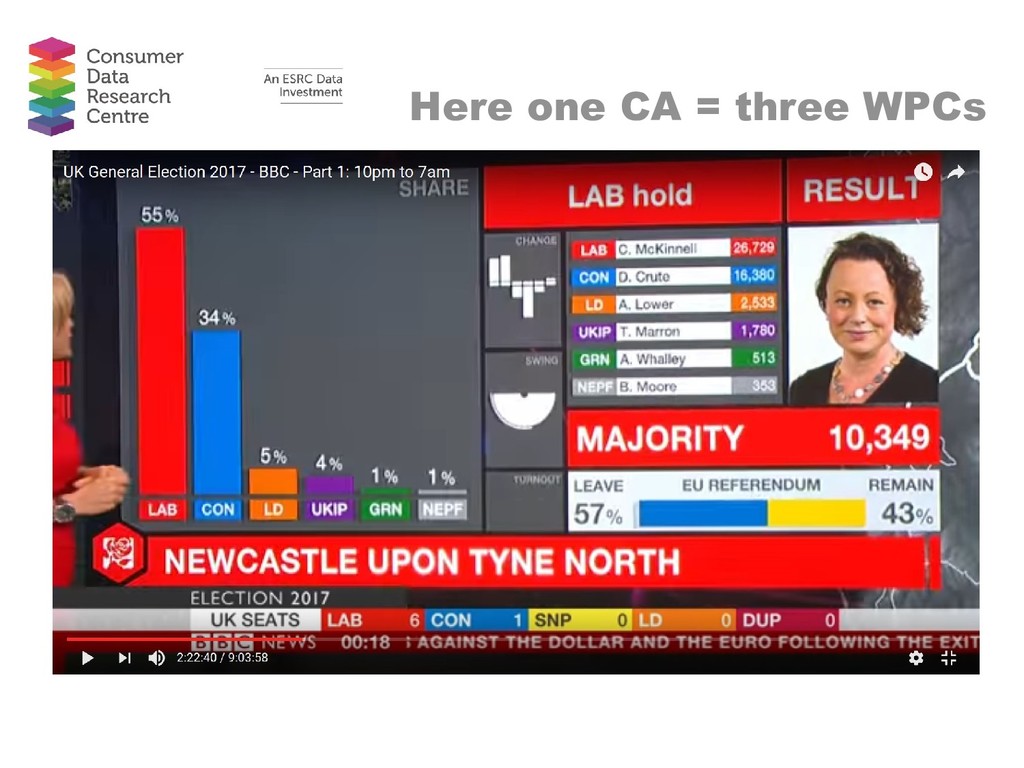
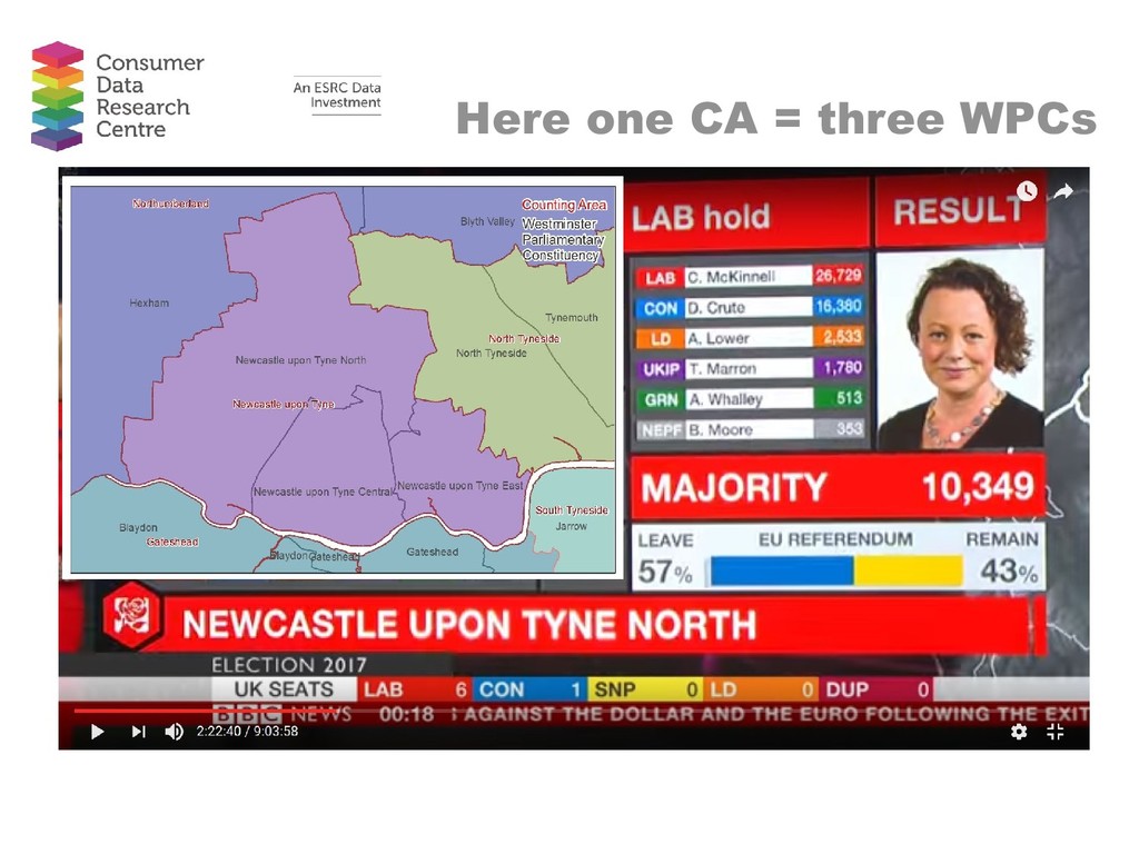
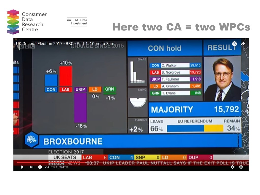
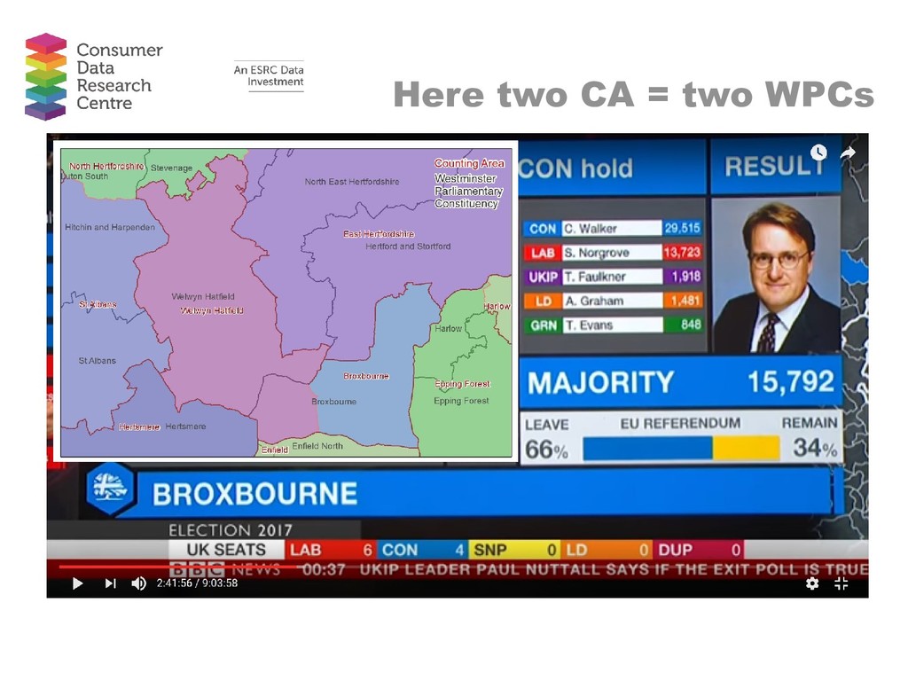
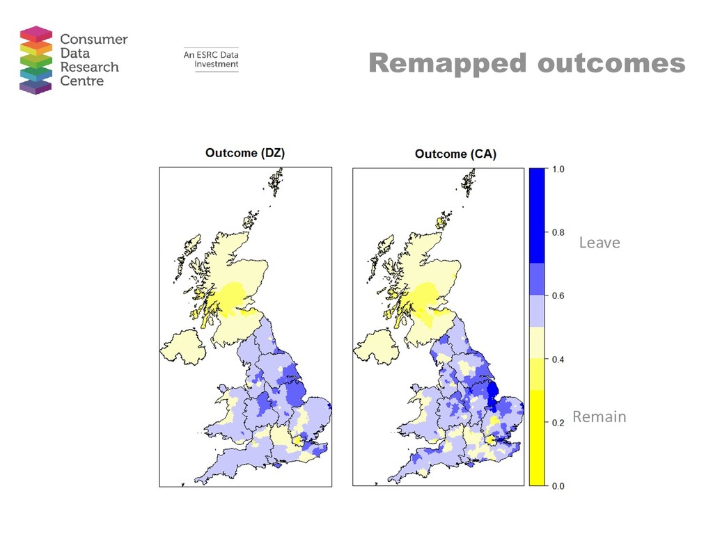
Abstract: There is currently much discussion and hype around the use of big data to provide insight in to a range of phenomena, from consumer behaviour to travel patterns. In this talk, I move away from discussion of big and emerging data to focus on recent work using what I loosely term ‘novel’ data. These are novel in the sense that they are data which are not routinely used in academia but which can provide insight in to local level phenomena and spatial patterns. I provide two substantive examples. The first dataset comes from a commercial provider and reports the characteristics of properties in the sales and rentals market. I use these data to assess local variation in house prices and in rent/price ratios. The second dataset is provided by the UK Government’s e-petitions website. I use these data to estimate the Brexit referendum vote share for Westminster Parliamentary Constituencies and to create a classification of Constituencies based on the types of petitions constituents sign. In both examples I utilise techniques often used on big datasets alongside more conventional techniques. Maps are used as a key tool for interpreting local level variations in both cases. The overall aim of this talk is to highlight that there are a wide range of data available which can provide insight in to spatial patterns which are not routinely used in research. Once we stop worrying about finding big datasets to solve problems, we can focus on applying useful techniques to the range of novel datasets available to us.

Transcript

1. Using Novel Data to Provide Local Insights Nik Lomax University of Leeds Royal Statistical Society | Leeds | 5 June 2019 @niklomax
2. Rationale • Much of the current discussion in data analytics is about ‘Big Data’ and Big Data methods • There is a lot of information out there which is very useful for research, but isn’t necessarily big data • I argue that we should use a looser term: ‘Novel Data’ to provide more flexibility • The bonus is that much of these data have spatial attributes
3. Motivation • Vision for research does not always equal reality • A ‘Medium Data Toolkit’ instead of ‘Big Data’ Source: Soundararaj, B., Cheshire, J. and Longley, P. (2019) Medium Data Toolkit - A Case study on Smart Street Sensor Project. Presentation at GISRUK, Newcastle, 24-26 April.
4. Motivation • As a Geographer, always looking for the spatial dimension to explain phenomena Source: Lomax (2019) What the UK population will look like by 2061 under hard, soft or no Brexit scenarios, The Conversation, https://bit.ly/2YUzwCT
5. Motivation • As a Geographer, always looking for the spatial dimension to explain phenomena Source: Lomax (2019) What the UK population will look like by 2061 under hard, soft or no Brexit scenarios, The Conversation, https://bit.ly/2YUzwCT
6. Motivation • People engage with spatial information • And there is plenty of it Source: Adcock and Lomax (2018) https://maps.cdrc.ac.uk/#/geodemographics/vulnerability/
7. Examples 1. A dataset from a commercial provider and reports the characteristics of properties in the sales and rentals market. Used to assess local variation in rental prices and in calculating rent/price ratios. 2. A dataset from the UK Government’s e- petitions website. Used to estimate the Brexit referendum vote share for Westminster Parliamentary Constituencies and to create a classification of Constituencies.
8. Example 1: Sales and rental data A mass market appraisal of the rental market Calculating rent/price ratio for English housing sub‐markets using matched sales and rental data
9. Data (are inherently spatial) • Rental data from online property search engine Zoopla, cleaned and supplied by When Fresh • 652,454 listings in 2014 and 552,459 in 2015 After cleaning n= 1,063,419 • Range of attributes including listing price, number of beds, type of property • Important to note that listing price ≠ final rental price
10. Introduction • Mass appraisal of house sales market well established • Needed for levying of local property taxes • Well established field in the literature • Broad approaches to appraisals: • (hedonic) valuation models • cost models (based on the materials, design and labour used) • use of comparable sales data • land value estimations
11. Introduction • Far less emphasis on mass market appraisal in rental market • But necessary to place a rental value on a property that reflects current market conditions • Has received little academic study • Primarily due to lack of available data on such transactions
12. Introduction • Banzhaf and Farooque (2013) rental values correlate with access to public goods and income levels in Los Angeles • Löchl (2010) accessibility and travel time most important for explaining rents in Zurich • Fuss and Koller (2016) neighbouring property price is most important using hedonic models for Zurich • Baron and Kaplan (2010) impact of ‘studentification’ on rent is negative in Haifa • Prunty (2016) difference in hedonic features in comparative study of New York and California • McCord et al (2014) use GWR, find a high level of segmentation across localised pockets of the Belfast rental market
13. Rationale and contribution • A lack of insight hampers commercial organisations and local and national governments in understanding rental market. • We offer a practical guide for property professionals and academics wishing to undertake such appraisals and looking for guidance on the best methods to use. • We provide insight in to the property characteristics which most influence rental listing price.
14. Data • Rental data from online property search engine Zoopla, cleaned and supplied by WhenFresh • 652,454 listings in 2014 and 552,459 in 2015 After cleaning n= 1,063,419 • Range of attributes including listing price, number of beds, type of property • Important to note that listing price ≠ final rental price
15. Data • Additional environmental variables • Distance from railway station (DFT) • Access to Healthy Assets and Hazards (CDRC) • School performance (DfE) • ACORN – commercial geodemographic profile (CACI)
16. Methods 1. Quassi Poisson generalised linear model (GLM) 2. Machine learning algorithms • Tree based: gradient boost (GB) and Cubist • Specialist non-linear models: support vector machines (SVM) and multiple adaptive splines (MARS) 3. Practitioner based approach (PBA) • rental price is a summary of recently rented similar properties in neighbourhood
17. Experimental procedure • All methods are applied in a consistent manner akin to a moving window • Information from the previous 12 months used predict the out-of-sample rental prices 2014 2015 Jan Feb Mar Apr May Jun Jul Aug Sept Oct Nov Dec Jan Feb Mar Apr May Jun Jul Aug Sept Oct Nov Dec
18. GLM Results • quassi Poisson generalised linear model (GLM) used because: • skewed distribution of the rental price • possible over-dispersion • Essential step prior to Machine Learning – Does the data capture dynamics of the housing market in a sensible manner? • 63 variables • Squared correlation between observed and in-sample predicted r2 = 0.738 on log of rental price • r2 drops to 0.54 on original scale
19. GLM Results -0.05 -0.04 -0.03 -0.02 -0.01 0 0.01 0.02 0.03 Bungalow Detached Semi-detached Terraced Unknown Property type Attribute N/median estimate std error t Intercept 487253 6.451 0.0067 957.7 *** Flat 212275 Bungalow 11617 0.0073 0.0059 1.2 Detached 31996 0.0192 0.0037 5.2 *** Semi- detached 54410 -0.0463 0.0032 -14.5 *** Terraced 111087 -0.0185 0.0025 -7.4 *** Unknown 65868 0.0169 0.0026 6.4 ***
20. -0.2 0 0.2 0.4 0.6 0.8 1 1.2 1.4 2 Bedrooms 3 Bedrooms 4 Bedrooms 5 Bedrooms 6 and more Bedrooms Unknown Number of bedrooms Attribute N/median estimate std error t Intercept 487253 6.451 0.0067 957.7 *** 1 Bedroom 94379 2 Bedrooms 192236 0.2772 0.0024 116.8 *** 3 Bedrooms 123546 0.5157 0.0028 186.7 *** 4 Bedrooms 41505 0.7607 0.0033 228.6 *** 5 Bedrooms 12558 1.008 0.0043 235.7 *** 6 and more Bedrooms 7097 1.265 0.0051 248.3 *** Unknown 15932 -0.0881 0.005 -17.7 *** GLM Results
21. 0 0.1 0.2 0.3 0.4 0.5 0.6 0.7 2 Bathrooms 3 Bathrooms 4 Bathrooms 5 and more Bathrooms Unknown Number of bathrooms Attribute N/median estimate std error t Intercept 487253 6.451 0.0067 957.7 *** 1 Bathroom 194157 2 Bathrooms 45440 0.1314 0.0026 50.8 *** 3 Bathrooms 6767 0.3343 0.0047 71.2 *** 4 Bathrooms 1150 0.5347 0.0085 63.3 *** 5 and more Bathrooms 622 0.6633 0.0107 62 *** Unknown 239117 0.1169 0.0024 48.2 *** GLM Results
22. -0.1 -0.05 0 0.05 0.1 0.15 0.2 0.25 0.3 0.35 0.4 2 Reception rooms 3 Reception rooms 4 Reception rooms 5 and more Reception rooms Unknown Number of reception rooms Attribute N/median estimate std error t Intercept 487253 6.451 0.0067 957.7 *** 1 Reception room 159999 2 Reception rooms 41912 0.002 0.003 0.7 3 Reception rooms 4921 0.0681 0.006 11.4 *** 4 Reception rooms 723 0.2235 0.0113 19.8 *** 5 and more Reception rooms 191 0.3379 0.0189 17.9 *** Unknown 279507 -0.0333 0.0024 -13.9 *** GLM Results
23. -0.03 -0.02 -0.01 0 0.01 0.02 0.03 Month of listing Attribute N/median estimate std error t Intercept 487253 6.451 0.0067 957.7 *** January 50988 February 37309 -0.022 0.0036 -6.2 *** March 39601 -0.0179 0.0035 -5.1 *** April 38037 -0.0098 0.0035 -2.8 ** May 40414 0.0095 0.0034 2.8 ** June 42095 -0.009 0.0034 -2.7 ** July 44808 -0.0031 0.0033 -0.9 August 39791 0.0068 0.0035 2 * September 37994 -0.0041 0.0035 -1.2 October 43005 0.0086 0.0034 2.5 * November 42037 0.0238 0.0034 7 *** December 31174 0.0042 0.0038 1.1 GLM Results
24. -0.1 -0.08 -0.06 -0.04 -0.02 0 0.02 0.04 5 to 10 11 to 20 21 to 60 61 and more Unknown Webpage visits per day Attribute N/median estimate std error t Intercept 487253 6.451 0.0067 957.7 *** Up to 4 24094 5 to 10 14610 0.0244 0.0055 4.4 *** 11 to 20 23114 -0.0199 0.005 -3.9 *** 21 to 60 39969 -0.0469 0.0046 -10.3 *** 61 and more 29423 -0.0754 0.005 -15.2 *** Unknown 356043 0.023 0.0037 6.2 *** GLM Results
25. -0.45 -0.4 -0.35 -0.3 -0.25 -0.2 -0.15 -0.1 -0.05 0 Rising prosperity Comfortable communities Financially stretched Urban adversity Not private households ACORN not known Acorn classification Attribute N/median estimate std error t Intercept 487253 6.451 0.0067 957.7 *** Affluent achievers 60017 Rising prosperity 136624 -0.1961 0.0026 -74.5 *** Comfortable communities 98779 -0.2798 0.0028 -99.7 *** Financially stretched 92146 -0.3463 0.0031 -112.9 *** Urban adversity 96472 -0.4212 0.0031 -134.3 *** Not private households 3008 -0.0994 0.009 -11.1 *** ACORN not known 207 -0.1028 0.0274 -3.8 *** GLM Results
26. -0.35 -0.3 -0.25 -0.2 -0.15 -0.1 -0.05 0 Log Distance from the City of London Log Distance from railway station Geography Attribute N/median estimate std error t Intercept 487253 6.451 0.0067 957.7 *** Log Distance from the City of London 113.95km -0.2862 0.00079 -363.2 *** Log Distance from railway station 1.11km -0.0204 0.001 -20 *** GLM Results
27. -0.0005 0 0.0005 0.001 0.0015 0.002 0.0025 0.003 Retail health Access health Environment health Environment and amenity Attribute N/median estimate std error t Intercept 487253 6.451 0.0067 957.7 *** Retail health 30.53 0.0025 0.00005 52.2 *** Access health 7.21 -0.0001 0.00008 -1.9 Environmen t health 25.32 0.0004 0.00004 10.5 *** GLM Results
28. Access to Healthy Assets and Hazards (AHAH) Daras, Konstantinos; Green, Mark; Davies, Alec; Singleton, Alex; Barr, Benjamin. (2017).
29. -0.12 -0.1 -0.08 -0.06 -0.04 -0.02 0 Good Primary school Requires improvement Primary school Inadequate Primary school Primary school Ofsted score Attribute N/median estimate std error t Intercept 487253 6.451 0.0067 957.7 *** Outstanding Primary 91869 Good Primary 308287 -0.0487 0.0019 -26.2 *** Requires improveme nt Primary 79841 -0.0614 0.0026 -24 *** Inadequate Primary 7256 -0.0972 0.0071 -13.7 *** GLM Results
30. -0.14 -0.12 -0.1 -0.08 -0.06 -0.04 -0.02 0 Good Secondary school Requires improvement Secondary school Inadequate Secondary school Secondary school Ofsted score Attribute N/median estimate std error t Intercept 487253 6.451 0.0067 957.7 *** Outstanding Secondary 1119014 Good Secondary 245070 -0.076 0.0018 -43.2 *** Requires improvement Secondary 96715 -0.1047 0.0024 -44.6 *** Inadequate Secondary 26454 -0.1269 0.0044 -28.9 *** GLM Results
31. Machine Learning • Algorithms fitted within the machine learning paradigm of the caret package in R • Primarily tree based algorithms: 1. Gradient boost (GB) 2. Cubist • Specialist non-linear models: 3. Support vector machines (SVM) 4. Multiple adaptive splines (MARS)
32. Practitioner approach • Combines price of recently rented similar properties in neighbourhood • Comparable properties must be of the same property type, have the same number of bedrooms, bathrooms and reception rooms and be in the same ACORN group. • Inverse distance weight used (closer properties contribute more)
33. Results – comparing r2 Testing PBA GLM GB SVM Cubist MARS Ensemble Jan 0.55 0.56 0.62 0.56 0.65 0.47 0.67 Feb 0.53 0.55 0.61 0.57 0.64 0.50 0.65 Mar 0.48 0.49 0.52 0.48 0.56 0.43 0.57 Apr 0.52 0.55 0.58 0.55 0.65 0.47 0.65 May 0.41 0.44 0.48 0.44 0.50 0.39 0.51 Jun 0.53 0.59 0.63 0.60 0.67 0.52 0.68 Jul 0.55 0.58 0.66 0.61 0.66 0.53 0.69 Aug 0.51 0.53 0.58 0.56 0.62 0.48 0.63 Sep 0.52 0.57 0.64 0.57 0.68 0.51 0.69 Oct 0.49 0.56 0.59 0.57 0.63 0.49 0.64 Nov 0.52 0.57 0.63 0.54 0.64 0.48 0.66 Dec 0.51 0.56 0.61 0.57 0.66 0.51 0.67 ALL 0.51 0.54 0.59 0.55 0.63 0.48 0.64
34. Results – comparing median percentage prediction error Testing PBA GLM GB SVM Cubist MARS Ensemble Jan 7.95 16.62 16.07 13.80 13.59 20.73 13.44 Feb 8.17 16.55 15.22 13.30 13.46 20.66 13.04 Mar 8.35 16.28 15.24 13.32 13.22 20.66 13.14 Apr 8.47 15.83 15.00 13.13 13.31 20.49 12.95 May 8.62 15.94 14.85 12.99 13.04 20.01 13.32 Jun 8.82 16.02 15.07 13.39 13.36 19.83 13.04 Jul 9.23 15.68 14.82 12.97 12.91 19.69 12.87 Aug 9.26 15.70 14.74 13.02 12.90 19.92 12.91 Sep 9.26 15.12 14.40 12.55 12.38 19.25 12.40 Oct 9.80 16.14 15.17 13.40 13.39 19.67 13.39 Nov 9.95 16.70 15.76 13.83 13.89 19.64 14.46 Dec 9.73 15.77 14.76 13.20 12.35 19.36 13.00 ALL 9.07 16.04 15.11 13.25 13.18 20.01 13.06
35. Results – distribution of percentage error
36. Conclusions • What increases rental price (from GLM): • Number of rooms in the property • proximity to central London • Proximity to railway stations • being located in more affluent neighbourhoods • being close to local amenities • Being close to better performing schools
37. Conclusions • Practitioner approach produced appraisals that have much smaller percentage error whilst the other approaches have better r2 • Our preferred Machine Learning Algorithm is Cubist
38. And conclusions from the other study… • An investor with £10million to invest and looking to maximise their gross rental yield would, rather than investing in a couple of properties in West London, be better off investing in hundreds of properties in the less affluent areas of the Midlands and North.
39. Example 2: E-Petition Data Estimating the outcome of UKs referendum on EU membership using e-petition data and machine learning algorithms Classification of Westminster Parliamentary constituencies using e-petition data
40. Context • On 23 June 2016, 52% voted in favour of leaving the EU (turnout 72% of registered voters) • Results published for ‘Counting Areas’ • But not for Westminster Parliamentary Constituencies (WPCs) • WPCs are geography that elected members of Parliament are held to account by their constituents.
41. Our study uses e-petition data and machine learning algorithms to estimate the Leave vote percentage for Westminster Parliamentary Constituencies. Context “for the purpose of examining dyadic representation … results at the level of Westminster parliamentary constituencies would be far more useful than results from local authority areas.” (Hanretty 2017, p. 466) Hanretty, C. 2017. "Areal interpolation and the UK's referendum on EU membership." Journal of Elections, Public Opinion and Parties:1-18. doi: 10.1080/17457289.2017.1287081.
42. e-petitions (X data) • Hosted by UK Parliament • Create or sign a petition that asks for a change to the law or to government policy. • Use e-petitions between May 2015 to April 2016 (25 petitions) • JSON files of raw counts in WPCs • Size of WPC electorate varies from 22k to 110k • Normalise by dividing by the size of the 2015 electorate
43. e-petitions used
44. e-petitions: geography
45. Counting areas (Y data) • EU votes counted for Counting Areas (CAs) (380) • Same as Local Authority Districts (LADs) • ex Orkney/Shetland • Most political interest at Westminster Parliamentary Constituencies (WPCs) (650) • Some CAs are co-terminus with WPCs • Some LADs released counts for WPCs/Wards • Issue of allocation of postal votes to WPCs
46. Incompatible geographies • Referendums results from 382 CAs • E-petition counts from 632 WPCs (exclude NI) • A new geography needed where aggregations of CAs are the same as aggregations of WPCs • 173 Data Zones Description Number of DZ Number of CA Number of WPC An aggregation of CAs same as a WPC CA ≡ WPC 1 2 1 CA same as a WPC CA ≡ WPC 35 35 35 CA same as an aggregation of WPCs CA ≡ WPC 55 55 158 An aggregation of CAs same as an aggregation of WPCs CA ≡ WPC 82 288 438 Total 173 380 632
47. Here one CA = one WPC
48. Here one CA = one WPC
49. Here one CA = three WPCs
50. Here one CA = three WPCs
51. Here two CA = two WPCs
52. Here two CA = two WPCs
53. Remapped outcomes Remain Leave
54. Machine learning algorithms • Lazy Learners • K nearest neighbours • Self-organising maps • Characterised by capturing learning through a set of similarity relationships in multidimensional ‘space’
55. Machine learning algorithms • Divide and Conquer • Random forests • Gradient Boost Machines • Largely tree-based algorithms, consisting of nodes which act as routing paths leading to a leaf (with if-then conditions)
56. Machine learning algorithms • Regression • Support Vector Machines • Artificial Neural Networks • MARS (BagEarth) • Designed to capture non-linear relationships
57. Machine learning algorithms • Hybrid • Cubist • Combination of a tradition decision tree and regression equations • At the leaf there is an estimated regression equation rather than a constant.
58. Machine learning (approach) • Use caret package in R to optimise parameters • 10 fold cross-validation repeated 10 times • Learn on Data Zone geography - aggregate up both CAs and WPCs to DZs • Keep 20% (33) back for out-of-sample performance • Use best algorithm to predict on WPC geography
59. Machine learning (performance) Algorithm RMSE R2 Cubist 0.0224 0.971 Nnet 0.0270 0.959 SVM 0.0279 0.955 BagEarth 0.0296 0.949 Ranger 0.0378 0.945 GLM 0.0307 0.944 GBM 0.0382 0.926 kNN 0.0547 0.885 SOM 0.0642 0.759
60. Hanretty, C. 2017. "Areal interpolation and the UK's referendum on EU membership." Journal of Elections, Public Opinion and Parties:1-18. doi: 10.1080/17457289.2017.1287081. Comparison against other studies • Hanretty (2017) uses areal interpolation • Scaled Poisson regression incorporates demographic information from lower level geographies. • Estimated 400 WPCs voted Leave whilst 232 voted Remain • Demonstrates geographic distribution of signatures to a petition for a second referendum strongly associated with how constituencies voted in the actual referendum.
61. Comparison against other studies • Marriott (2017) uses a look-up table of WPCs to CAs and then a method to re-allocate votes to a WPC based on a ‘classification’ of each WPC. • Estimated a Leave vote for 403 WPCs (later updated to 400) Marriott, J. 2017 "EU Referendum 2016 #1 – How and why did Leave win and what does it mean for UK politics? (a 4-part special)." https://marriott- stats.com/nigels-blog/brexit-why-leave-won/.
62. Results (WPC)
63. Results (BREXIT) • Hard Remain = 201 • Hard Leave = 372 • Soft Remain = 29 • Soft Leave = 30
64. Discussion • WPCs are the democratic geography – MPs elected and represent their constituents • Largely confirms Hanretty’s and Marriot’s estimates • Signatories ≠ Electors • Method can be applied in different contexts • For example – plans to reduce the number of WPCs from 650 to 600
65. Conclusion • e-petition data is an informative and versatile source of information that gauges the political sentiment in a location • This sentiment can be used to infer other outcomes • Scope for political scientists to apply machine learning algorithms to gain confirmatory or alternative insight.
66. And conclusions from the other study… There are four distinct classes of Westminster Parliamentary Constituency Two liberal classes are identified that are concentrated in and around London, one conservative class to be found in the urban centres and a distinct class concerned with rural issues.
67. Final Conclusions • ‘Novel’ data is out there • It is useful and applicable to academic research • We should be doing interesting things with it • Don’t get hung up on ‘big data’! • Novel data often has a spatial dimension… • … which people can relate to
68. Links and reading Link to The Conversation article https://bit.ly/2YUzwCT https://bit.ly/2JTLt8t https://bit.ly/2MvtFCE https://bit.ly/2Z96j7d https://bit.ly/2Z6Meyp Link to CDRC Maps https://maps.cdrc.ac.uk
69. • Three-tier Data Access • Secure Facilities • Trusted Researchers • Governance • Safe results @niklomax Questions