iRIC MI

Transcript

1. iRIC V4 Release June 28, 2023 iRIC: International River Interface Cooperative International River Interface Cooperative, since 2010 “New Developments for iRIC-MI Model Coupling” Jonathan Nelson US Geological Survey- Ret’d Now at: River Mechanics, Inc Arvada, Colorado, USA Keisuke Inoue Mizuho Instrumentation and Research Tokyo, Japan Kazutake Asahi RiverLink Corporation Tokyo, Japan
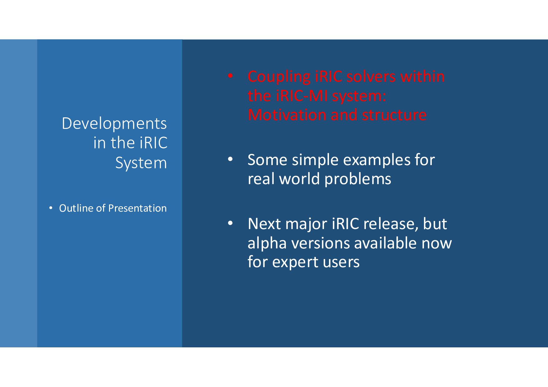
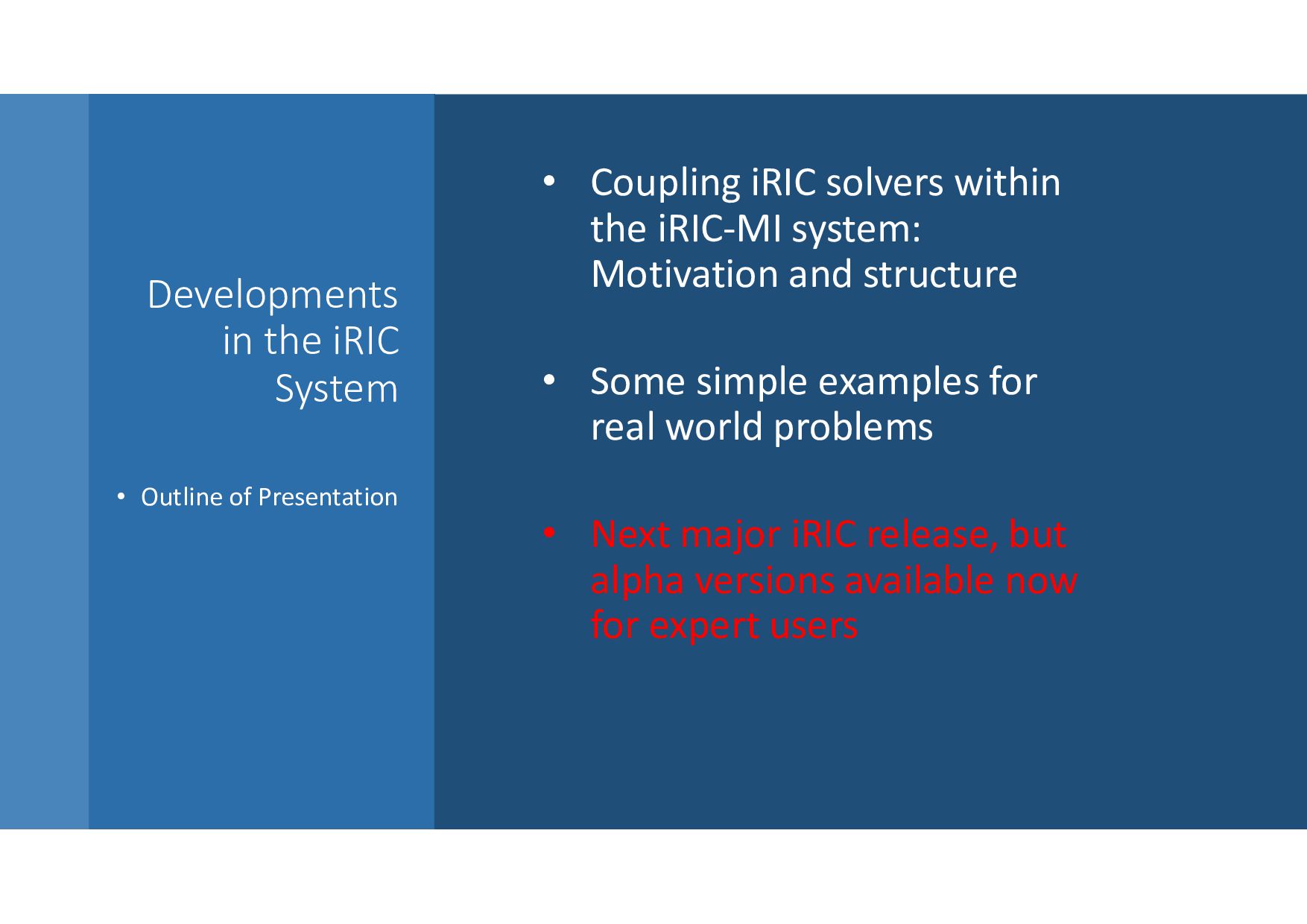
2. Developments in the iRIC System • Outline of Presentation • Coupling iRIC solvers within the iRIC-MI system: Motivation and structure • Some simple examples for real world problems • Next major iRIC release, but alpha versions available now for expert users
3. iRIC-MI = iRIC Model Interface • Platform to run solvers connected together • Similar to CommonMP and OpenMI but with several advantages: • Easy to use: iRIC GUI can be used to handle data • Development of model is easy • Runs on many platforms
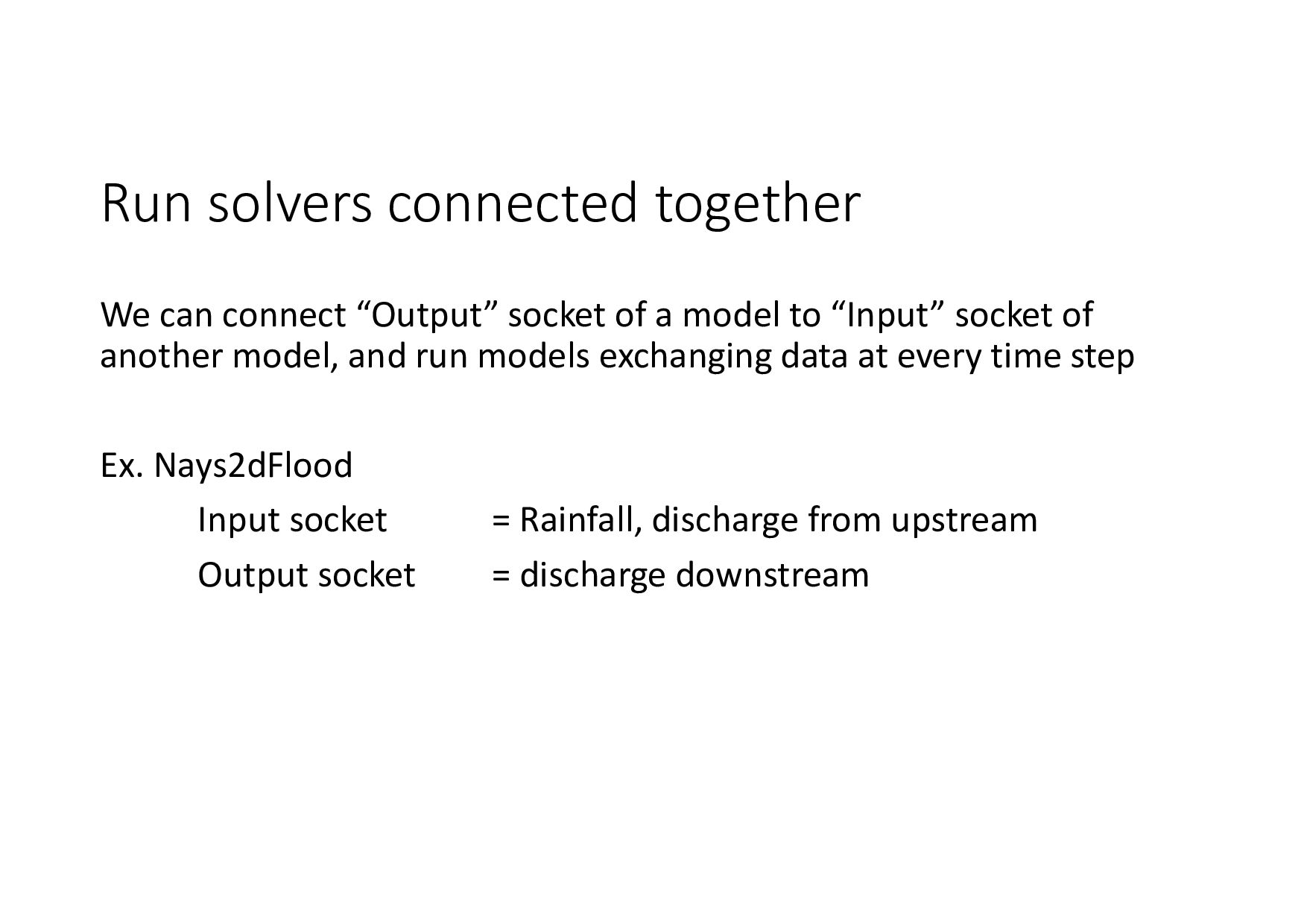
4. Run solvers connected together We can connect “Output” socket of a model to “Input” socket of another model, and run models exchanging data at every time step Ex. Nays2dFlood Input socket = Rainfall, discharge from upstream Output socket = discharge downstream
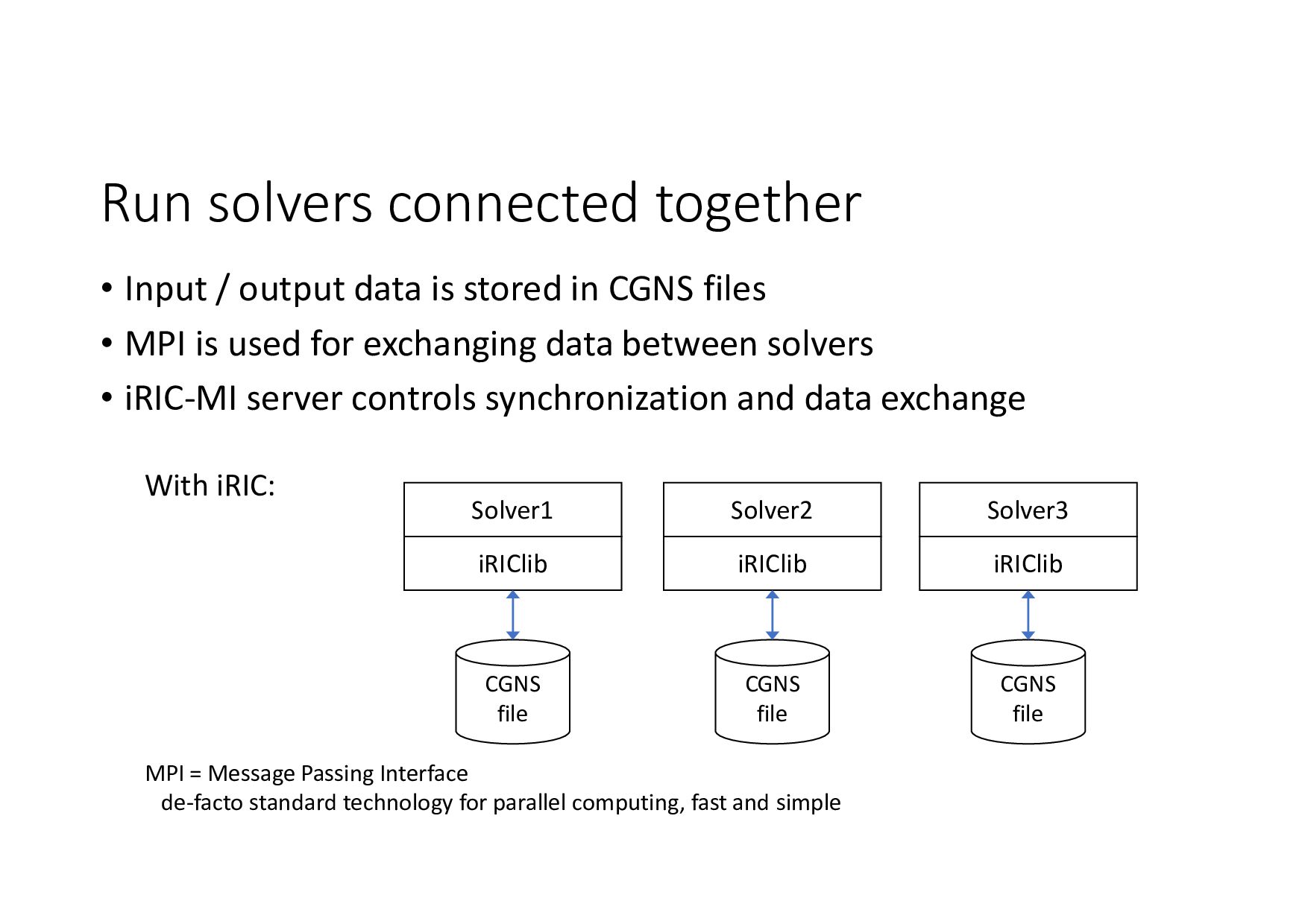
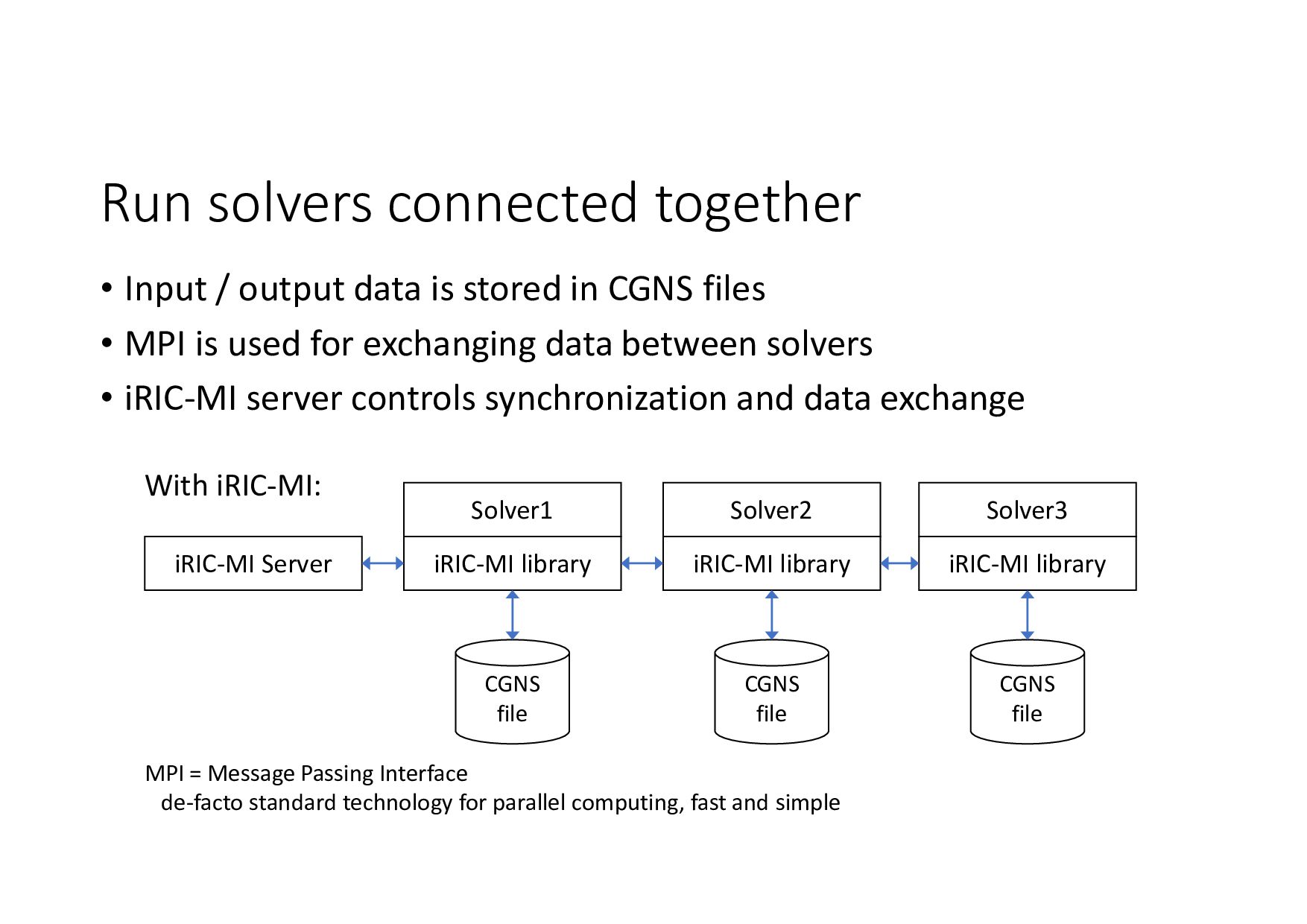
5. Run solvers connected together • Input / output data is stored in CGNS files • MPI is used for exchanging data between solvers • iRIC-MI server controls synchronization and data exchange iRIClib iRIClib iRIClib Solver1 Solver2 Solver3 CGNS file CGNS file CGNS file With iRIC: MPI = Message Passing Interface de-facto standard technology for parallel computing, fast and simple
6. Run solvers connected together • Input / output data is stored in CGNS files • MPI is used for exchanging data between solvers • iRIC-MI server controls synchronization and data exchange iRIC-MI library iRIC-MI library iRIC-MI library Solver1 Solver2 Solver3 iRIC-MI Server CGNS file CGNS file CGNS file With iRIC-MI: MPI = Message Passing Interface de-facto standard technology for parallel computing, fast and simple
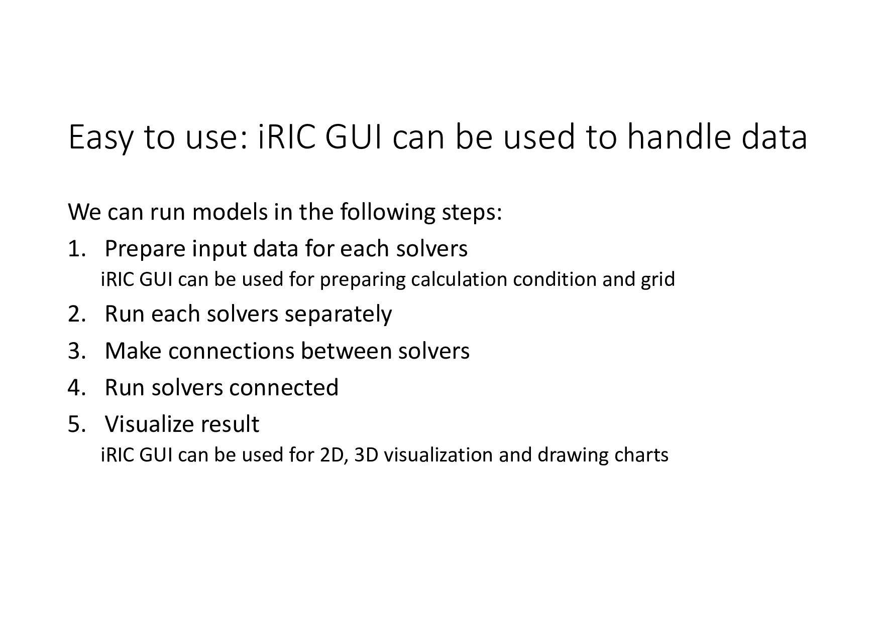
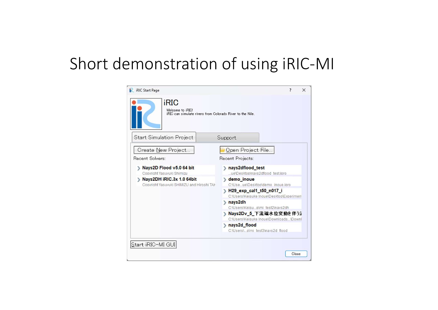
7. Easy to use: iRIC GUI can be used to handle data We can run models in the following steps: 1. Prepare input data for each solvers iRIC GUI can be used for preparing calculation condition and grid 2. Run each solvers separately 3. Make connections between solvers 4. Run solvers connected 5. Visualize result iRIC GUI can be used for 2D, 3D visualization and drawing charts
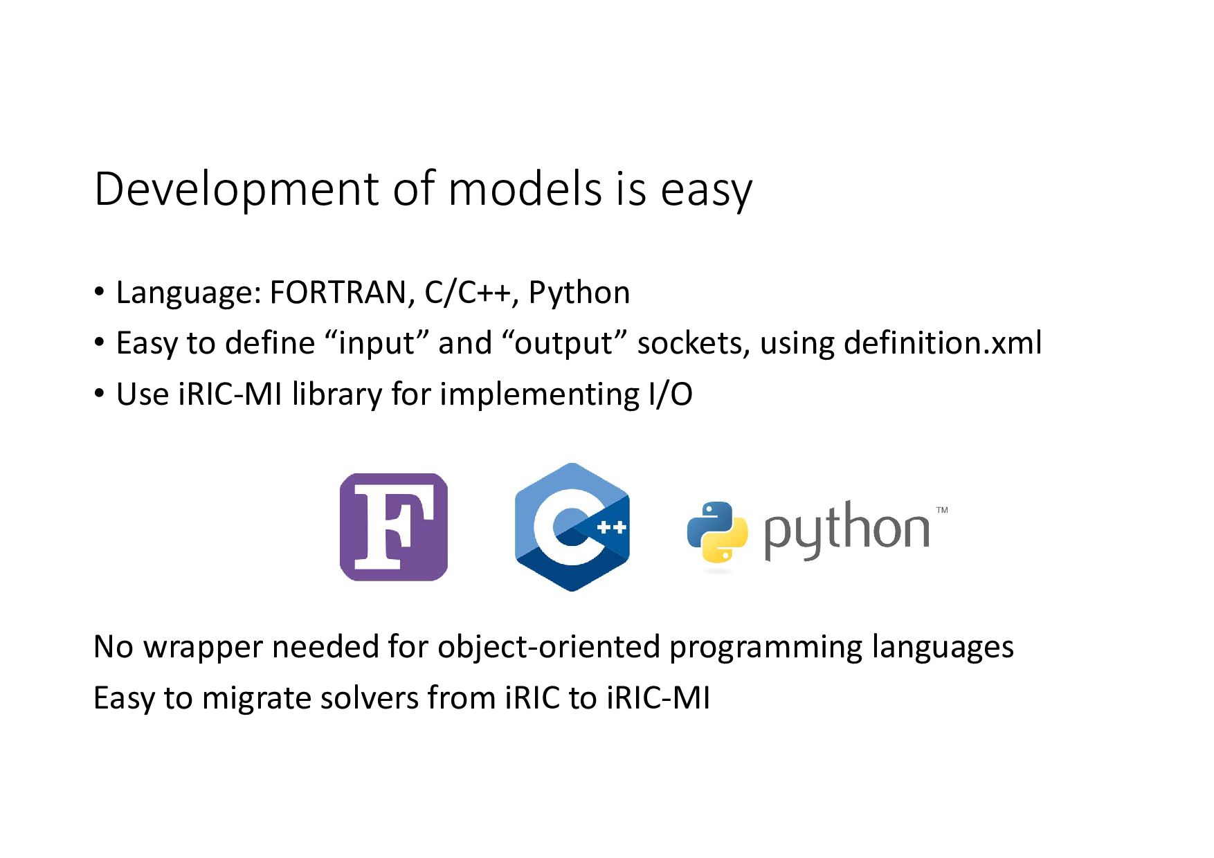
8. Development of models is easy • Language: FORTRAN, C/C++, Python • Easy to define “input” and “output” sockets, using definition.xml • Use iRIC-MI library for implementing I/O No wrapper needed for object-oriented programming languages Easy to migrate solvers from iRIC to iRIC-MI
9. Runs on many platforms • PCs with Windows / Mac OS X / Linux • Virtual machines in Cloud of Amazon, Google, or MS. • Super computers  Can be used to solve real problems
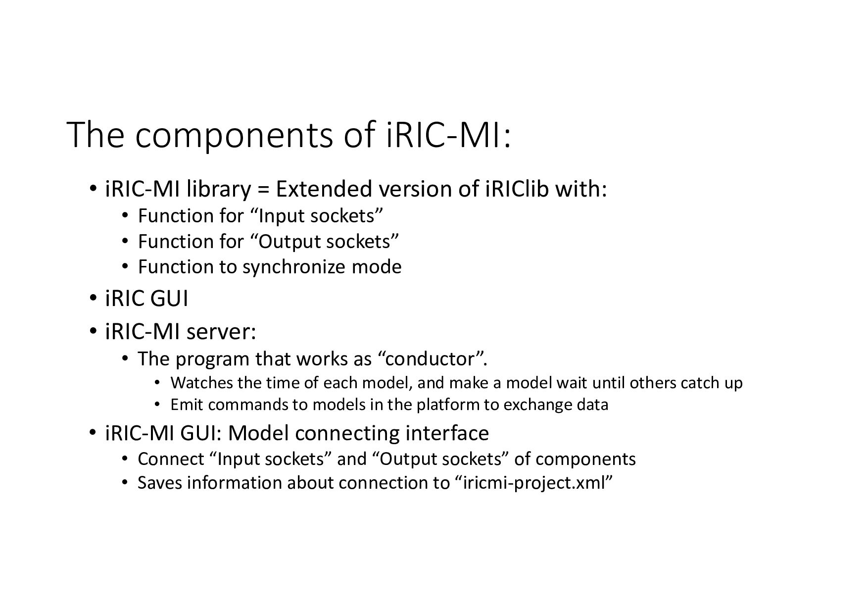
10. The components of iRIC-MI: • iRIC-MI library = Extended version of iRIClib with: • Function for “Input sockets” • Function for “Output sockets” • Function to synchronize mode • iRIC GUI • iRIC-MI server: • The program that works as “conductor”. • Watches the time of each model, and make a model wait until others catch up • Emit commands to models in the platform to exchange data • iRIC-MI GUI: Model connecting interface • Connect “Input sockets” and “Output sockets” of components • Saves information about connection to “iricmi-project.xml”
11. Short demonstration of using iRIC-MI
12. iRIC-MI Characteristics • End user ready (no programming required, this is not just another package of callable routines for programmers) • Interface support for setting up all coupled models (each model has its own interface, but they all look consistent- learn one, not 20) • No limit on type or number of coupled models running concurrently
13. iRIC-MI Characteristics (cont) • No limit on multiple-core usage by individual models or overall • XML for defining model inputs/outputs and coupling scheme (invisible to user, but makes new model inclusion straightforward) • Any coordinate system: structured (including non- orthogonal, multigrid, etc) and unstructured (holes, local resolution, any element shape) • Coupling for global values, boundary conditions, and/or individual grid nodes, faces, or cells
14. Developments in the iRIC System • Outline of Presentation • Coupling iRIC solvers within the iRIC-MI system: Motivation and structure • Some simple examples for real world problems • Next major iRIC release, but alpha versions available now for expert users
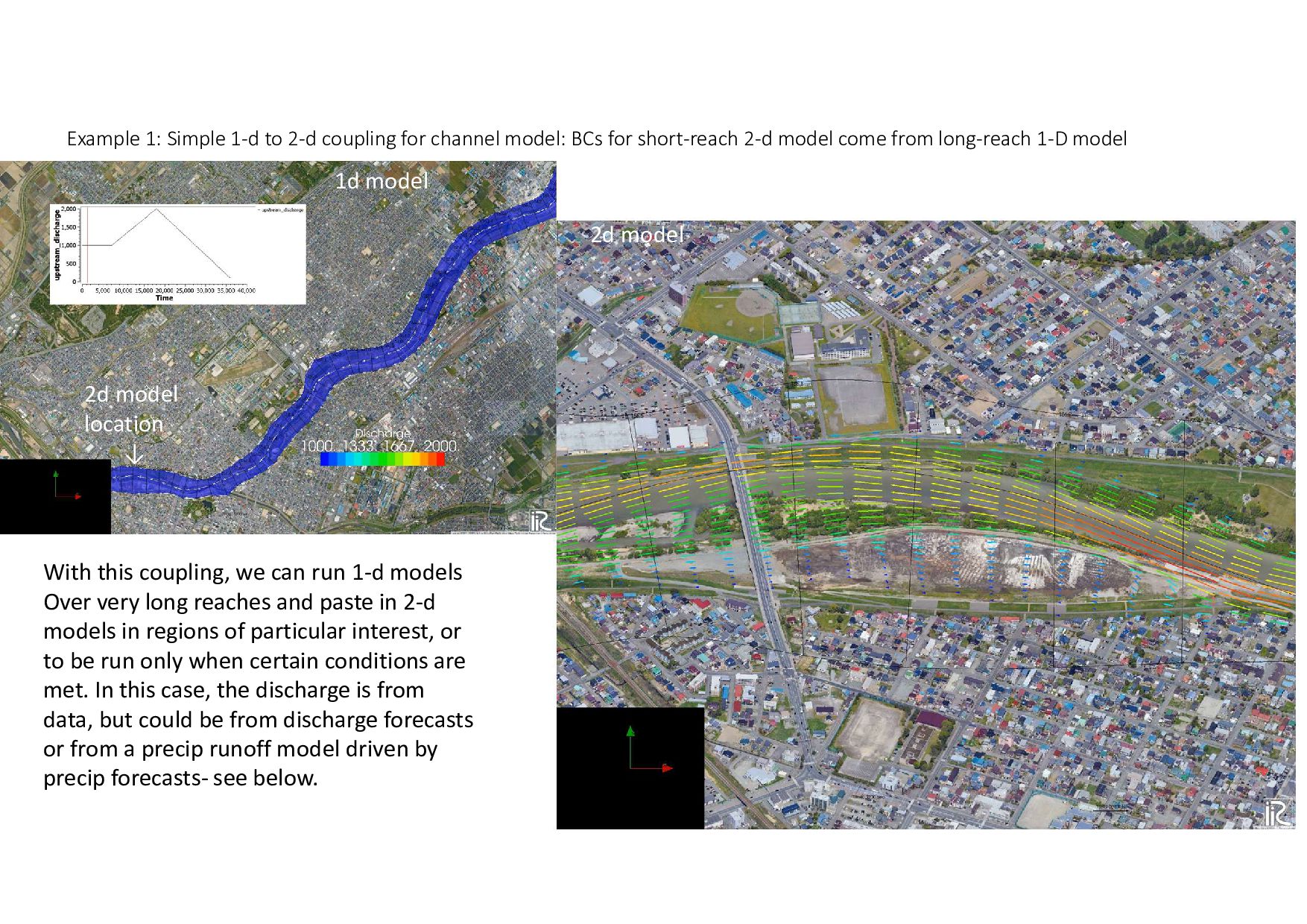
15. Example 1: Simple 1-d to 2-d coupling for channel model: BCs for short-reach 2-d model come from long-reach 1-D model With this coupling, we can run 1-d models Over very long reaches and paste in 2-d models in regions of particular interest, or to be run only when certain conditions are met. In this case, the discharge is from data, but could be from discharge forecasts or from a precip runoff model driven by precip forecasts- see below. 2d model location ↓ 2d model 1d model
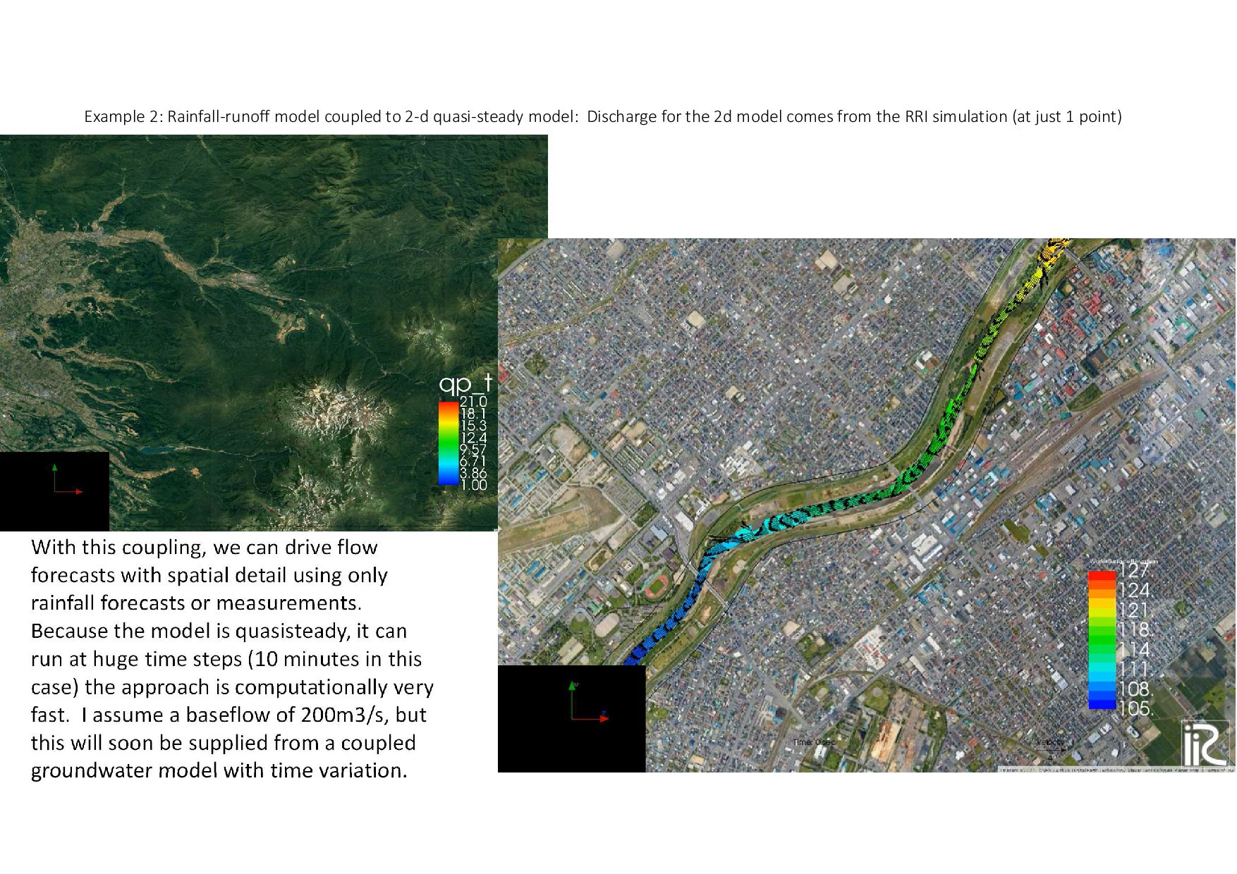
16. Example 2: Rainfall-runoff model coupled to 2-d quasi-steady model: Discharge for the 2d model comes from the RRI simulation (at just 1 point) With this coupling, we can drive flow forecasts with spatial detail using only rainfall forecasts or measurements. Because the model is quasisteady, it can run at huge time steps (10 minutes in this case) the approach is computationally very fast. I assume a baseflow of 200m3/s, but this will soon be supplied from a coupled groundwater model with time variation.
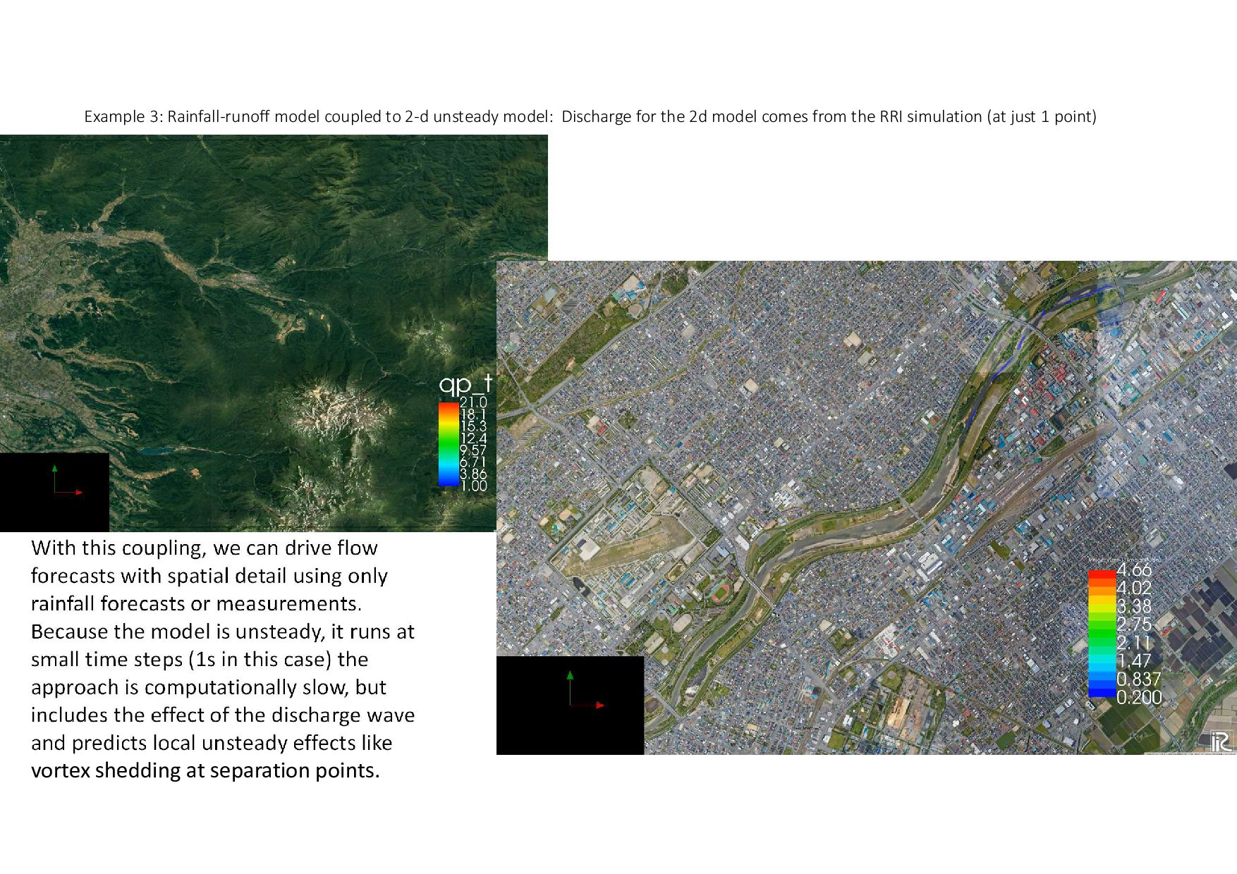
17. Example 3: Rainfall-runoff model coupled to 2-d unsteady model: Discharge for the 2d model comes from the RRI simulation (at just 1 point) With this coupling, we can drive flow forecasts with spatial detail using only rainfall forecasts or measurements. Because the model is unsteady, it runs at small time steps (1s in this case) the approach is computationally slow, but includes the effect of the discharge wave and predicts local unsteady effects like vortex shedding at separation points.
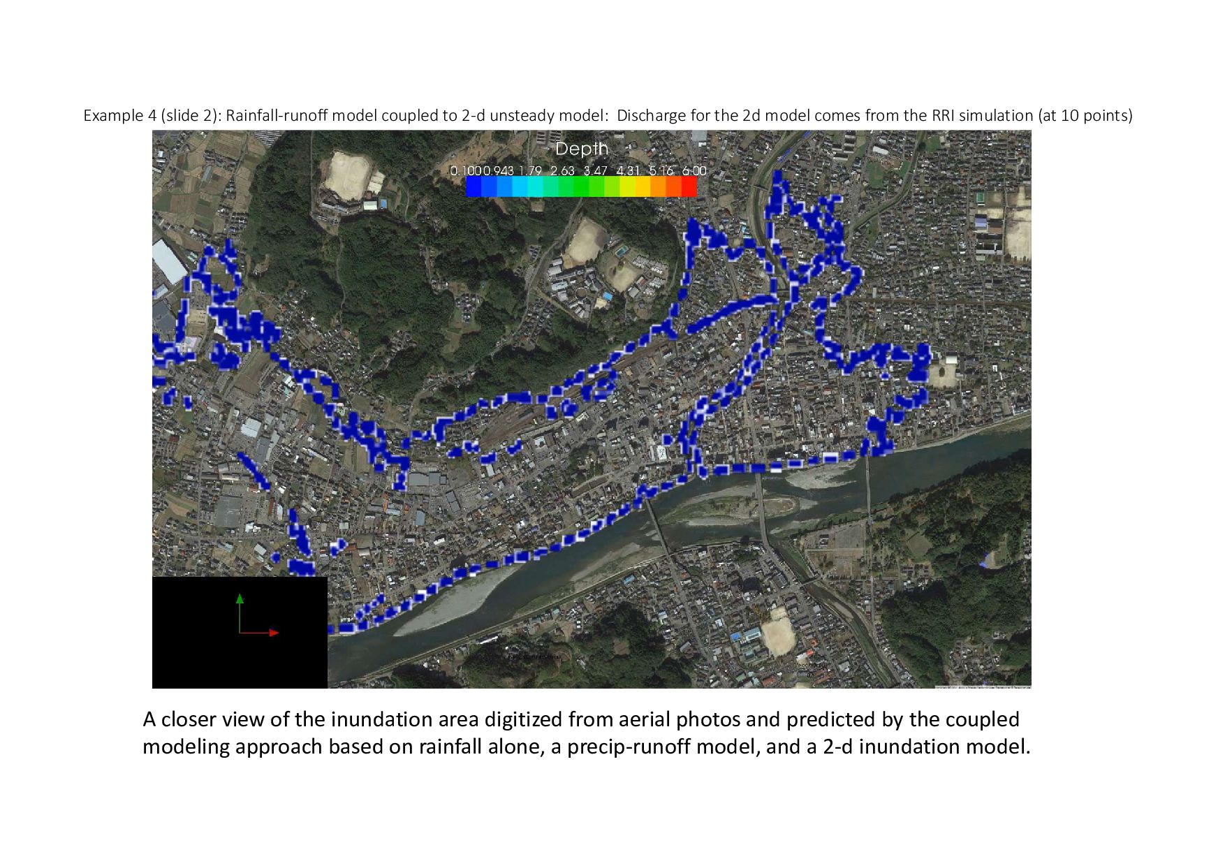
18. Example 3: Rainfall-runoff model coupled to 2-d unsteady model: Discharge for the 2d model comes from the RRI simulation (at 10 points) Here’s a more realistic case where we couple the rainfall runoff model to a 2-d fully unsteady urban inundation model at 10 upstream points. In the coupling system, this is still only boundary condition coupling, although the inundation model also handles in-domain rainfall. In this case, our colleague Kazutake Asahi digitized the locus of maximum inundation for this three-day flood (blue dashes) which can be compared to the prediction. Not bad, considering no calibration.
19. Example 4 (slide 2): Rainfall-runoff model coupled to 2-d unsteady model: Discharge for the 2d model comes from the RRI simulation (at 10 points) A closer view of the inundation area digitized from aerial photos and predicted by the coupled modeling approach based on rainfall alone, a precip-runoff model, and a 2-d inundation model.
20. Future Visions • Making solvers more reusable and customizable • New applications: • Environmental evaluation • Coupled models of rain-fall, river flows, ground water • Geochemistry • Machine learning • Easier for new developers to join the community
21. Developments in the iRIC System • Outline of Presentation • Coupling iRIC solvers within the iRIC-MI system: Motivation and structure • Some simple examples for real world problems • Next major iRIC release, but alpha versions available now for expert users
22. 22 Questions? www.i-ric.org