Assimilation of image structures

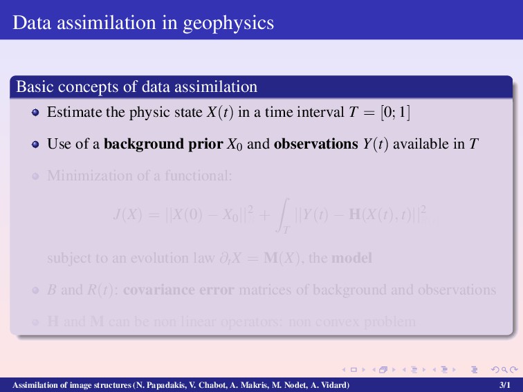
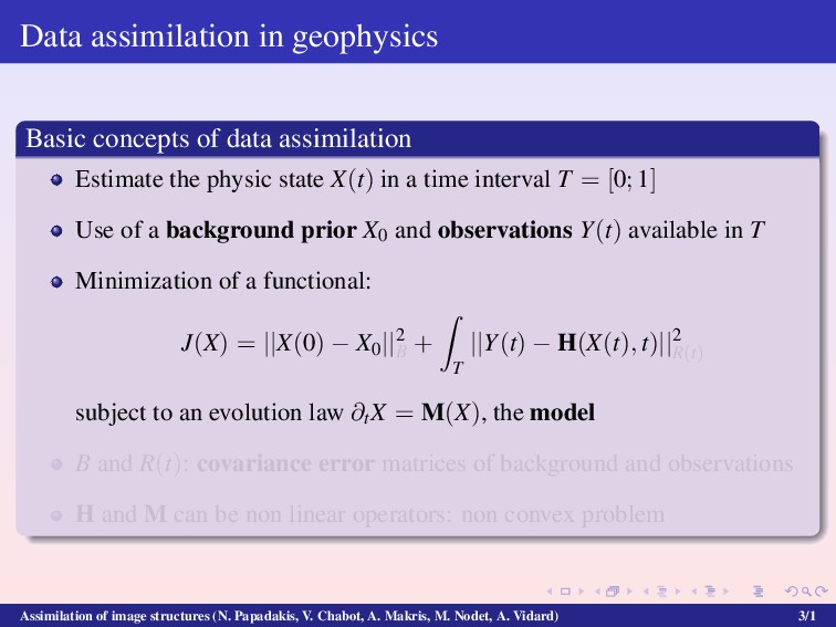
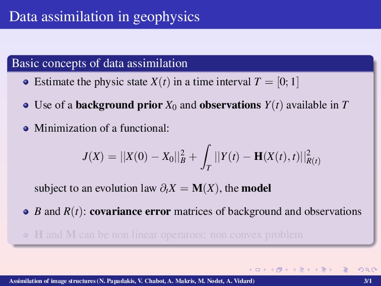
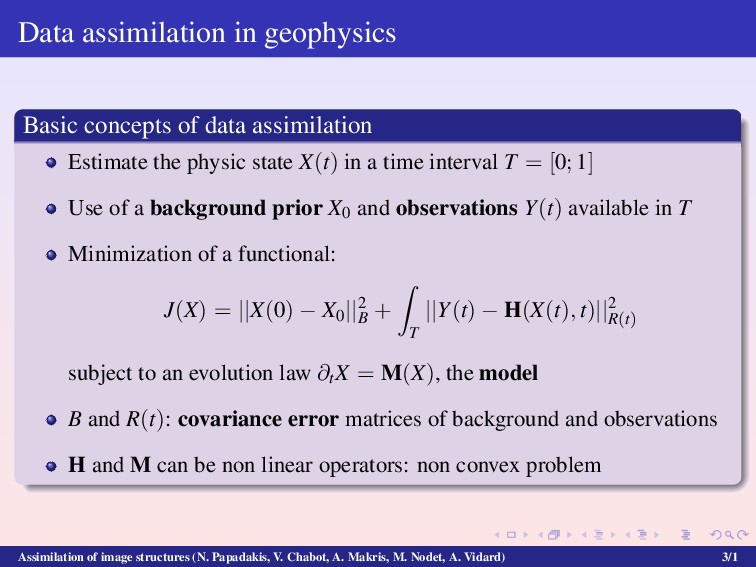
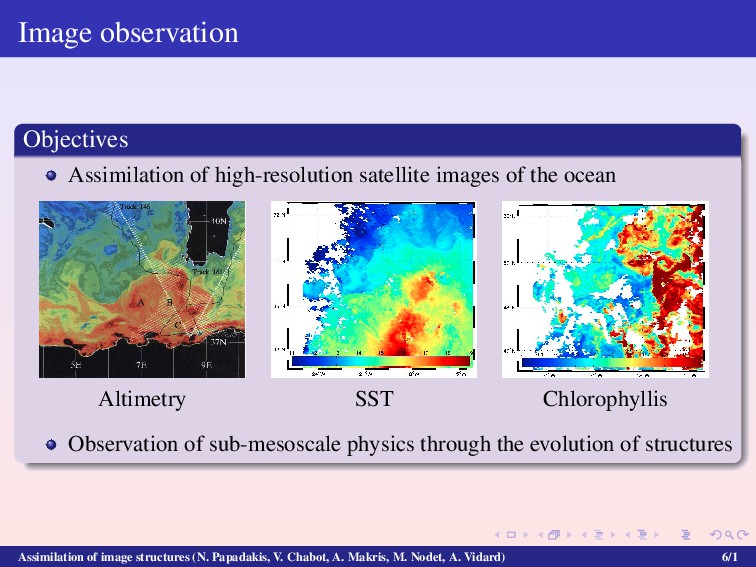
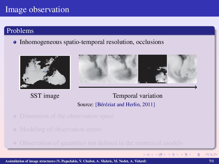
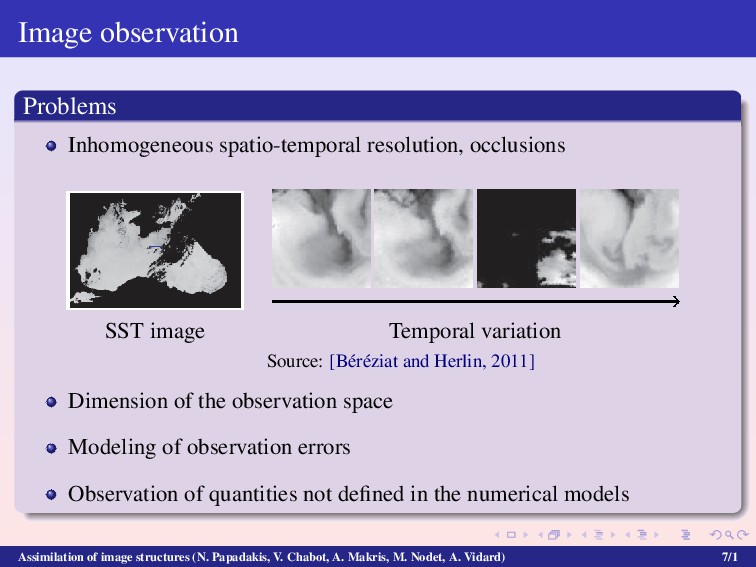
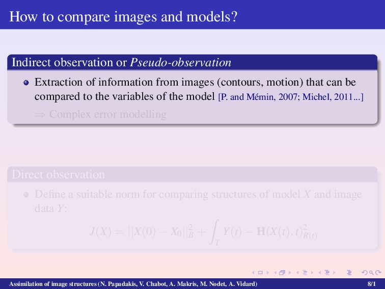
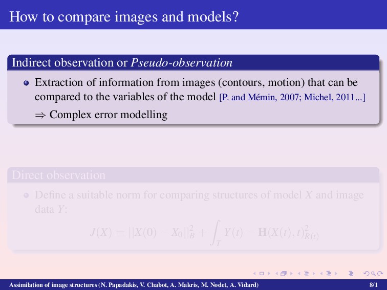
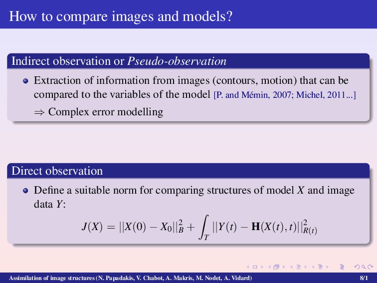
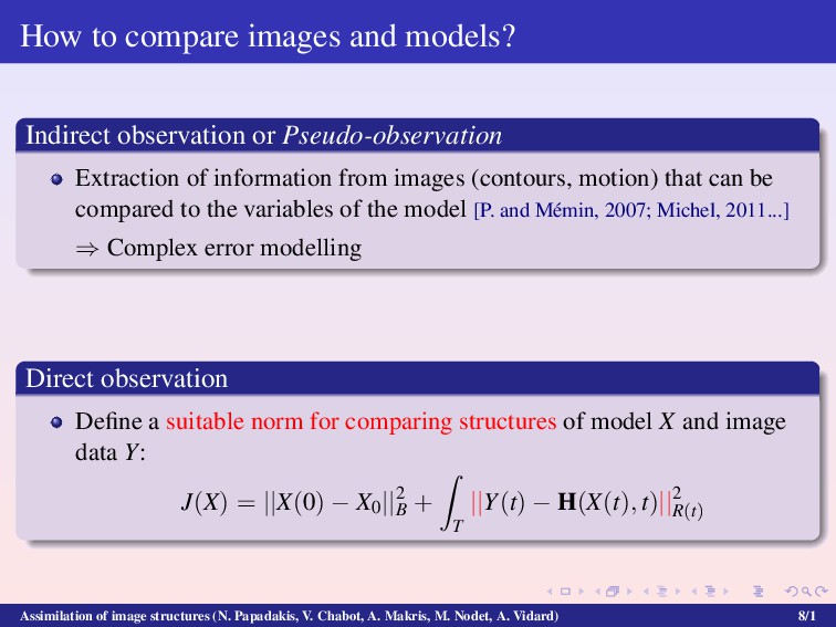
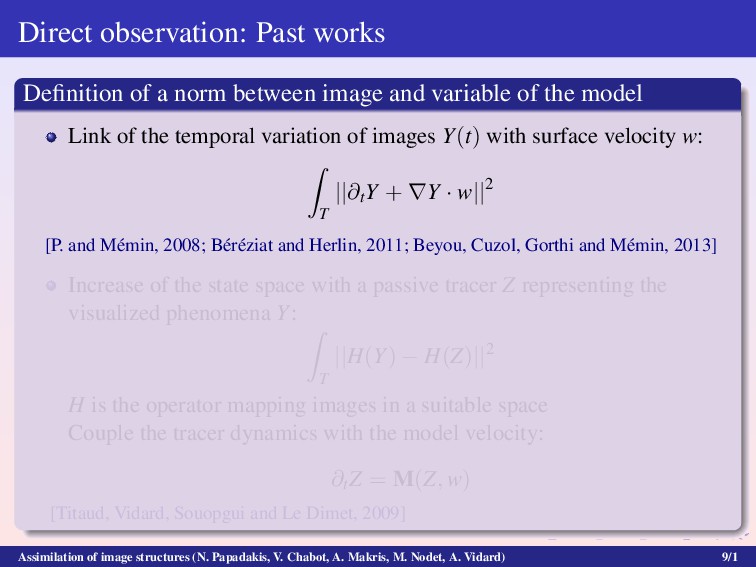
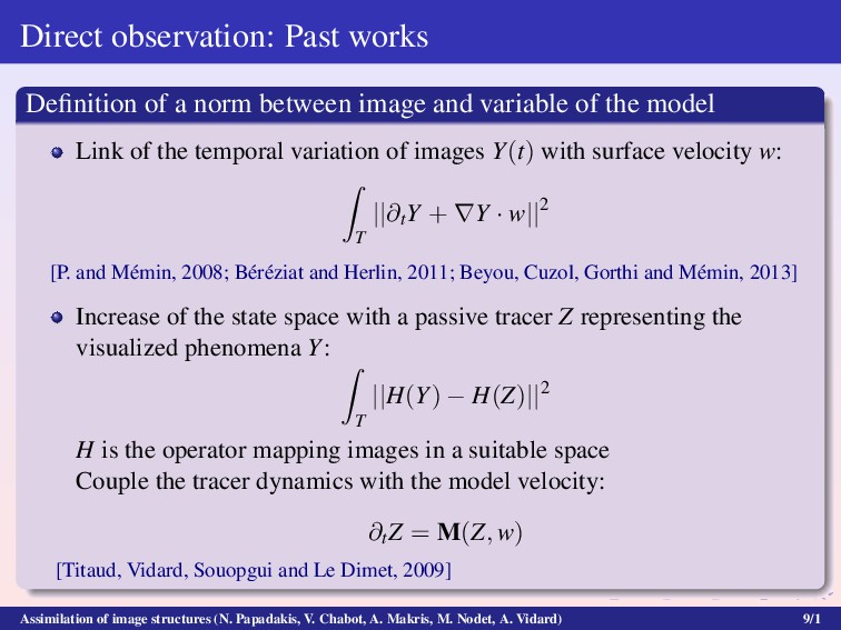
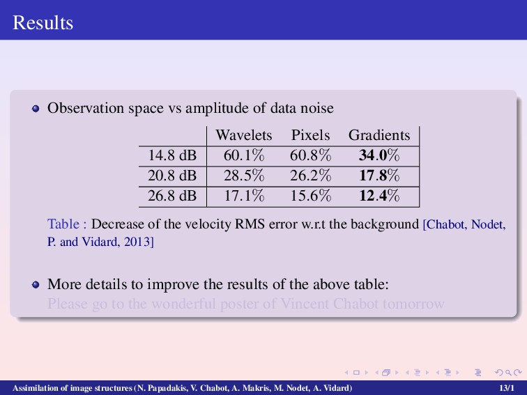
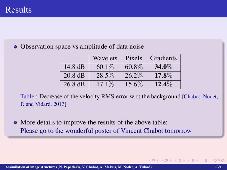
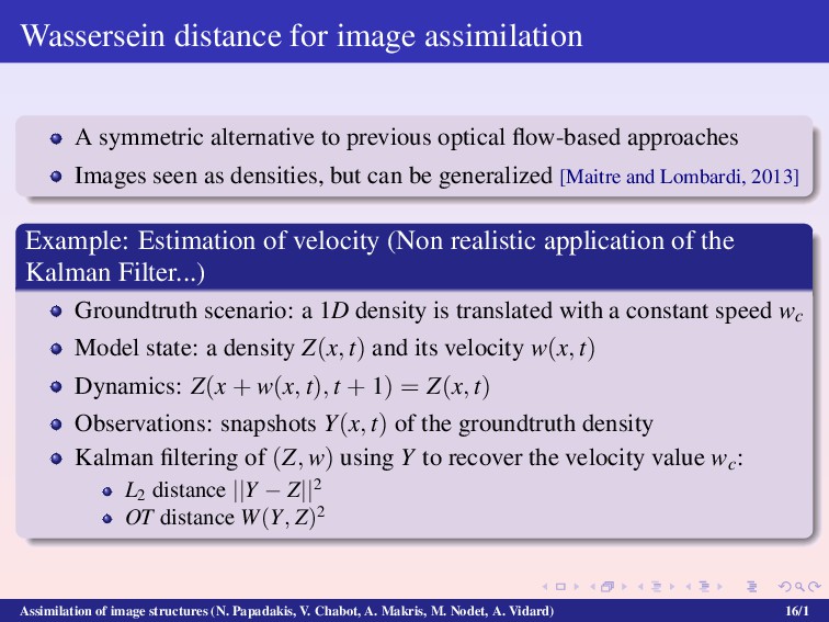
This work reviews some recent works on assimilation of structures contained in satellite images of the ocean. Image assimilation consists in controlling the state of a numerical model using the spatio-temporal information of image sequences. The main issue is to measure the difference between an ideal image provided by the model and a satellite image. We therefore propose different kind of metrics between images that allow a better assimilation of image structure information.

Transcript

1. Assimilation of image structures Nicolas Papadakis1,2, Vincent Chabot2, Alexandros Makris2, M¨ aelle Nodet2, Arthur Vidard2 1 CNRS, Institut de Math´ ematiques de Bordeaux 2 ´ Equipe Moise, Laboratoire Jean Kuntzmann/Inria Grenoble GRETSI September 5th 2013 Assimilation of image structures (N. Papadakis, V. Chabot, A. Makris, M. Nodet, A. Vidard)
2. Scientific context Theme: Mathematical and numerical methods for modelling and understanding the evolution of geophysic fluids: ocean, atmosphere, ice... Applications: short and long term forecasting, risk analysis... Today’s subject: Use of satellite images to monitor numerical models of the ocean: data assimilation Assimilation of image structures (N. Papadakis, V. Chabot, A. Makris, M. Nodet, A. Vidard) 1/1
3. Scientific context Theme: Mathematical and numerical methods for modelling and understanding the evolution of geophysic fluids: ocean, atmosphere, ice... Applications: short and long term forecasting, risk analysis... Today’s subject: Use of satellite images to monitor numerical models of the ocean: data assimilation Assimilation of image structures (N. Papadakis, V. Chabot, A. Makris, M. Nodet, A. Vidard) 1/1
4. Overview Assimilation of image structures (N. Papadakis, V. Chabot, A. Makris, M. Nodet, A. Vidard)
5. Overview Assimilation of image structures (N. Papadakis, V. Chabot, A. Makris, M. Nodet, A. Vidard)
6. Data assimilation in geophysics Three main types of information Numerical model: temporal evolution of physical quantities (velocity, temperature, sea height, pressure...) Observations: obtained from stations, ballons, driftbuoys (sparse/dense in space/time) Uncertaincies: confidence in the background, the model and the observations (modelling of mesurement errors) Assimilation of image structures (N. Papadakis, V. Chabot, A. Makris, M. Nodet, A. Vidard) 2/1
7. Data assimilation in geophysics Basic concepts of data assimilation Estimate the physic state X(t) in a time interval T = [0; 1] Use of a background prior X0 and observations Y(t) available in T Minimization of a functional: J(X) = ||X(0) − X0||2 B + T ||Y(t) − H(X(t), t)||2 R(t) subject to an evolution law ∂tX = M(X), the model B and R(t): covariance error matrices of background and observations H and M can be non linear operators: non convex problem Assimilation of image structures (N. Papadakis, V. Chabot, A. Makris, M. Nodet, A. Vidard) 3/1
8. Data assimilation in geophysics Basic concepts of data assimilation Estimate the physic state X(t) in a time interval T = [0; 1] Use of a background prior X0 and observations Y(t) available in T Minimization of a functional: J(X) = ||X(0) − X0||2 B + T ||Y(t) − H(X(t), t)||2 R(t) subject to an evolution law ∂tX = M(X), the model B and R(t): covariance error matrices of background and observations H and M can be non linear operators: non convex problem Assimilation of image structures (N. Papadakis, V. Chabot, A. Makris, M. Nodet, A. Vidard) 3/1
9. Data assimilation in geophysics Basic concepts of data assimilation Estimate the physic state X(t) in a time interval T = [0; 1] Use of a background prior X0 and observations Y(t) available in T Minimization of a functional: J(X) = ||X(0) − X0||2 B + T ||Y(t) − H(X(t), t)||2 R(t) subject to an evolution law ∂tX = M(X), the model B and R(t): covariance error matrices of background and observations H and M can be non linear operators: non convex problem Assimilation of image structures (N. Papadakis, V. Chabot, A. Makris, M. Nodet, A. Vidard) 3/1
10. Data assimilation in geophysics Basic concepts of data assimilation Estimate the physic state X(t) in a time interval T = [0; 1] Use of a background prior X0 and observations Y(t) available in T Minimization of a functional: J(X) = ||X(0) − X0||2 B + T ||Y(t) − H(X(t), t)||2 R(t) subject to an evolution law ∂tX = M(X), the model B and R(t): covariance error matrices of background and observations H and M can be non linear operators: non convex problem Assimilation of image structures (N. Papadakis, V. Chabot, A. Makris, M. Nodet, A. Vidard) 3/1
11. Sequential data assimilation [Kalman, 1960] Assimilation of image structures (N. Papadakis, V. Chabot, A. Makris, M. Nodet, A. Vidard) 4/1
12. Sequential data assimilation [Kalman, 1960] Assimilation of image structures (N. Papadakis, V. Chabot, A. Makris, M. Nodet, A. Vidard) 4/1
13. Sequential data assimilation [Kalman, 1960] Assimilation of image structures (N. Papadakis, V. Chabot, A. Makris, M. Nodet, A. Vidard) 4/1
14. Sequential data assimilation [Kalman, 1960] Assimilation of image structures (N. Papadakis, V. Chabot, A. Makris, M. Nodet, A. Vidard) 4/1
15. Sequential data assimilation [Kalman, 1960] Assimilation of image structures (N. Papadakis, V. Chabot, A. Makris, M. Nodet, A. Vidard) 4/1
16. Sequential data assimilation [Kalman, 1960] Assimilation of image structures (N. Papadakis, V. Chabot, A. Makris, M. Nodet, A. Vidard) 4/1
17. Sequential data assimilation [Kalman, 1960] Assimilation of image structures (N. Papadakis, V. Chabot, A. Makris, M. Nodet, A. Vidard) 4/1
18. Sequential data assimilation [Kalman, 1960] Assimilation of image structures (N. Papadakis, V. Chabot, A. Makris, M. Nodet, A. Vidard) 4/1
19. Variational data assimilation [Le Dimet, 1982] Assimilation of image structures (N. Papadakis, V. Chabot, A. Makris, M. Nodet, A. Vidard) 5/1
20. Variational data assimilation [Le Dimet, 1982] Assimilation of image structures (N. Papadakis, V. Chabot, A. Makris, M. Nodet, A. Vidard) 5/1
21. Variational data assimilation [Le Dimet, 1982] Assimilation of image structures (N. Papadakis, V. Chabot, A. Makris, M. Nodet, A. Vidard) 5/1
22. Variational data assimilation [Le Dimet, 1982] Assimilation of image structures (N. Papadakis, V. Chabot, A. Makris, M. Nodet, A. Vidard) 5/1
23. Variational data assimilation [Le Dimet, 1982] Assimilation of image structures (N. Papadakis, V. Chabot, A. Makris, M. Nodet, A. Vidard) 5/1
24. Variational data assimilation [Le Dimet, 1982] Assimilation of image structures (N. Papadakis, V. Chabot, A. Makris, M. Nodet, A. Vidard) 5/1
25. Overview Assimilation of image structures (N. Papadakis, V. Chabot, A. Makris, M. Nodet, A. Vidard)
26. Image observation Objectives Assimilation of high-resolution satellite images of the ocean Altimetry SST Chlorophyllis Observation of sub-mesoscale physics through the evolution of structures Assimilation of image structures (N. Papadakis, V. Chabot, A. Makris, M. Nodet, A. Vidard) 6/1
27. Image observation Problems Inhomogeneous spatio-temporal resolution, occlusions SST image Temporal variation Source: [B´ er´ eziat and Herlin, 2011] Dimension of the observation space Modeling of observation errors Observation of quantities not defined in the numerical models Assimilation of image structures (N. Papadakis, V. Chabot, A. Makris, M. Nodet, A. Vidard) 7/1
28. Image observation Problems Inhomogeneous spatio-temporal resolution, occlusions SST image Temporal variation Source: [B´ er´ eziat and Herlin, 2011] Dimension of the observation space Modeling of observation errors Observation of quantities not defined in the numerical models Assimilation of image structures (N. Papadakis, V. Chabot, A. Makris, M. Nodet, A. Vidard) 7/1
29. How to compare images and models? Indirect observation or Pseudo-observation Extraction of information from images (contours, motion) that can be compared to the variables of the model [P. and M´ emin, 2007; Michel, 2011...] ⇒ Complex error modelling Direct observation Define a suitable norm for comparing structures of model X and image data Y: J(X) = ||X(0) − X0||2 B + T Y(t) − H(X(t), t)2 R(t) Assimilation of image structures (N. Papadakis, V. Chabot, A. Makris, M. Nodet, A. Vidard) 8/1
30. How to compare images and models? Indirect observation or Pseudo-observation Extraction of information from images (contours, motion) that can be compared to the variables of the model [P. and M´ emin, 2007; Michel, 2011...] ⇒ Complex error modelling Direct observation Define a suitable norm for comparing structures of model X and image data Y: J(X) = ||X(0) − X0||2 B + T Y(t) − H(X(t), t)2 R(t) Assimilation of image structures (N. Papadakis, V. Chabot, A. Makris, M. Nodet, A. Vidard) 8/1
31. How to compare images and models? Indirect observation or Pseudo-observation Extraction of information from images (contours, motion) that can be compared to the variables of the model [P. and M´ emin, 2007; Michel, 2011...] ⇒ Complex error modelling Direct observation Define a suitable norm for comparing structures of model X and image data Y: J(X) = ||X(0) − X0||2 B + T ||Y(t) − H(X(t), t)||2 R(t) Assimilation of image structures (N. Papadakis, V. Chabot, A. Makris, M. Nodet, A. Vidard) 8/1
32. How to compare images and models? Indirect observation or Pseudo-observation Extraction of information from images (contours, motion) that can be compared to the variables of the model [P. and M´ emin, 2007; Michel, 2011...] ⇒ Complex error modelling Direct observation Define a suitable norm for comparing structures of model X and image data Y: J(X) = ||X(0) − X0||2 B + T ||Y(t) − H(X(t), t)||2 R(t) Assimilation of image structures (N. Papadakis, V. Chabot, A. Makris, M. Nodet, A. Vidard) 8/1
33. Overview Assimilation of image structures (N. Papadakis, V. Chabot, A. Makris, M. Nodet, A. Vidard)
34. Direct observation: Past works Definition of a norm between image and variable of the model Link of the temporal variation of images Y(t) with surface velocity w: T ||∂tY + ∇Y · w||2 [P. and M´ emin, 2008; B´ er´ eziat and Herlin, 2011; Beyou, Cuzol, Gorthi and M´ emin, 2013] Increase of the state space with a passive tracer Z representing the visualized phenomena Y: T ||H(Y) − H(Z)||2 H is the operator mapping images in a suitable space Couple the tracer dynamics with the model velocity: ∂tZ = M(Z, w) [Titaud, Vidard, Souopgui and Le Dimet, 2009] Assimilation of image structures (N. Papadakis, V. Chabot, A. Makris, M. Nodet, A. Vidard) 9/1
35. Direct observation: Past works Definition of a norm between image and variable of the model Link of the temporal variation of images Y(t) with surface velocity w: T ||∂tY + ∇Y · w||2 [P. and M´ emin, 2008; B´ er´ eziat and Herlin, 2011; Beyou, Cuzol, Gorthi and M´ emin, 2013] Increase of the state space with a passive tracer Z representing the visualized phenomena Y: T ||H(Y) − H(Z)||2 H is the operator mapping images in a suitable space Couple the tracer dynamics with the model velocity: ∂tZ = M(Z, w) [Titaud, Vidard, Souopgui and Le Dimet, 2009] Assimilation of image structures (N. Papadakis, V. Chabot, A. Makris, M. Nodet, A. Vidard) 9/1
36. Direct observation: Past works Compare its amplitude to the image intensity (pixels, curvelets) [Titaud, Vidard, Souopgui and Le Dimet, 2009] Sequence of fluorescein images CORIOLIS experimental turntable (Grenoble, France) Assimilation of image structures (N. Papadakis, V. Chabot, A. Makris, M. Nodet, A. Vidard) 10/1
37. Direct observation: Current works Compare its position to the image level lines (gradients, normals) [Ba and Fablet, 2010; Chabot, Nodet, P. and Vidard, 2013] Sequence of fluorescein images CORIOLIS experimental turntable (Grenoble, France) Assimilation of image structures (N. Papadakis, V. Chabot, A. Makris, M. Nodet, A. Vidard) 10/1
38. Experimental framework State variable: X = {2D velocity w = (u, v), sea height h, tracer Z} 2D Shallow-water model:    ∂tu − (f + ζ)v + ∂xB = −r∗u + κ∆u ∂tv + (f + ζ)u + ∂yB = −r∗v + κ∆v ∂th + ∂x(hu) + ∂y(hv) = 0. Coupling the tracer evolution with the model velocities: ∂tZ + u∂xZ + v∂yZ = ν∆Z Assimilation of image structures (N. Papadakis, V. Chabot, A. Makris, M. Nodet, A. Vidard) 11/1
39. Experimental framework State variable: X = {2D velocity w = (u, v), sea height h, tracer Z} 2D Shallow-water model:    ∂tu − (f + ζ)v + ∂xB = −r∗u + κ∆u ∂tv + (f + ζ)u + ∂yB = −r∗v + κ∆v ∂th + ∂x(hu) + ∂y(hv) = 0. Coupling the tracer evolution with the model velocities: ∂tZ + u∂xZ + v∂yZ = ν∆Z Assimilation of image structures (N. Papadakis, V. Chabot, A. Makris, M. Nodet, A. Vidard) 11/1
40. Experimental framework State variable: X = {2D velocity w = (u, v), sea height h, tracer Z} 2D Shallow-water model:    ∂tu − (f + ζ)v + ∂xB = −r∗u + κ∆u ∂tv + (f + ζ)u + ∂yB = −r∗v + κ∆v ∂th + ∂x(hu) + ∂y(hv) = 0. Coupling the tracer evolution with the model velocities: ∂tZ + u∂xZ + v∂yZ = ν∆Z Assimilation of image structures (N. Papadakis, V. Chabot, A. Makris, M. Nodet, A. Vidard) 11/1
41. Observation space and error modelling Study of different observation spaces for comparing images: Data compression: wavelet transform T (Z) and coefficient thresholding Structure position: gradients ∇Z, normals ∇Z/||∇Z|| Twin experiments to study the robustness to data noise Modeling of additive or multiplicative noise into the observation covariance matrices R Groundtruth Additive noise Multiplicative noise Assimilation of image structures (N. Papadakis, V. Chabot, A. Makris, M. Nodet, A. Vidard) 12/1
42. Observation space and error modelling Study of different observation spaces for comparing images: Data compression: wavelet transform T (Z) and coefficient thresholding Structure position: gradients ∇Z, normals ∇Z/||∇Z|| Twin experiments to study the robustness to data noise Modeling of additive or multiplicative noise into the observation covariance matrices R Groundtruth Additive noise Multiplicative noise Assimilation of image structures (N. Papadakis, V. Chabot, A. Makris, M. Nodet, A. Vidard) 12/1
43. Results Observation space vs amplitude of data noise Wavelets Pixels Gradients 14.8 dB 60.1% 60.8% 34.0% 20.8 dB 28.5% 26.2% 17.8% 26.8 dB 17.1% 15.6% 12.4% Table : Decrease of the velocity RMS error w.r.t the background [Chabot, Nodet, P. and Vidard, 2013] More details to improve the results of the above table: Please go to the wonderful poster of Vincent Chabot tomorrow Assimilation of image structures (N. Papadakis, V. Chabot, A. Makris, M. Nodet, A. Vidard) 13/1
44. Results Observation space vs amplitude of data noise Wavelets Pixels Gradients 14.8 dB 60.1% 60.8% 34.0% 20.8 dB 28.5% 26.2% 17.8% 26.8 dB 17.1% 15.6% 12.4% Table : Decrease of the velocity RMS error w.r.t the background [Chabot, Nodet, P. and Vidard, 2013] More details to improve the results of the above table: Please go to the wonderful poster of Vincent Chabot tomorrow Assimilation of image structures (N. Papadakis, V. Chabot, A. Makris, M. Nodet, A. Vidard) 13/1
45. Overview Assimilation of image structures (N. Papadakis, V. Chabot, A. Makris, M. Nodet, A. Vidard)
46. Optimal transport Let ρ0 and ρ1 be two positive densities M is the the set of transport maps pushing forward ρ0 to ρ1: ρ0(x) = ρ1(M(x))| det(∂M(x))| Define a cost C(M) associated to each transport map M ∈ M: C(M) = ||x − M(x)||2 Wasserstein distance W2(ρ0, ρ1): minimal cost C(M∗) Optimal transport map M∗: unique Associated geodesic path: trajectories in straight lines Assimilation of image structures (N. Papadakis, V. Chabot, A. Makris, M. Nodet, A. Vidard) 14/1
47. Optimal transport Let ρ0 and ρ1 be two positive densities M is the the set of transport maps pushing forward ρ0 to ρ1: ρ0(x) = ρ1(M(x))| det(∂M(x))| Define a cost C(M) associated to each transport map M ∈ M: C(M) = ||x − M(x)||2 Wasserstein distance W2(ρ0, ρ1): minimal cost C(M∗) Optimal transport map M∗: unique Associated geodesic path: trajectories in straight lines Assimilation of image structures (N. Papadakis, V. Chabot, A. Makris, M. Nodet, A. Vidard) 14/1
48. Optimal transport Let ρ0 and ρ1 be two positive densities M is the the set of transport maps pushing forward ρ0 to ρ1: ρ0(x) = ρ1(M(x))| det(∂M(x))| Define a cost C(M) associated to each transport map M ∈ M: C(M) = ||x − M(x)||2 Wasserstein distance W2(ρ0, ρ1): minimal cost C(M∗) Optimal transport map M∗: unique Associated geodesic path: trajectories in straight lines Assimilation of image structures (N. Papadakis, V. Chabot, A. Makris, M. Nodet, A. Vidard) 14/1
49. Optimal transport Wasserstein distance for comparing images L2 interpolation W2 interpolation + A pertinent distance for comparing image structures - Computational cost for signal of dimension > 1 Assimilation of image structures (N. Papadakis, V. Chabot, A. Makris, M. Nodet, A. Vidard) 15/1
50. Optimal transport Wasserstein distance for comparing images L2 interpolation W2 interpolation + A pertinent distance for comparing image structures - Computational cost for signal of dimension > 1 Assimilation of image structures (N. Papadakis, V. Chabot, A. Makris, M. Nodet, A. Vidard) 15/1
51. Wassersein distance for image assimilation A symmetric alternative to previous optical flow-based approaches Images seen as densities, but can be generalized [Maitre and Lombardi, 2013] Example: Estimation of velocity (Non realistic application of the Kalman Filter...) Groundtruth scenario: a 1D density is translated with a constant speed wc Model state: a density Z(x, t) and its velocity w(x, t) Dynamics: Z(x + w(x, t), t + 1) = Z(x, t) Observations: snapshots Y(x, t) of the groundtruth density Kalman filtering of (Z, w) using Y to recover the velocity value wc: L2 distance ||Y − Z||2 OT distance W(Y, Z)2 Assimilation of image structures (N. Papadakis, V. Chabot, A. Makris, M. Nodet, A. Vidard) 16/1
52. Wassersein distance for image assimilation A symmetric alternative to previous optical flow-based approaches Images seen as densities, but can be generalized [Maitre and Lombardi, 2013] Example: Estimation of velocity (Non realistic application of the Kalman Filter...) Groundtruth scenario: a 1D density is translated with a constant speed wc Model state: a density Z(x, t) and its velocity w(x, t) Dynamics: Z(x + w(x, t), t + 1) = Z(x, t) Observations: snapshots Y(x, t) of the groundtruth density Kalman filtering of (Z, w) using Y to recover the velocity value wc: L2 distance ||Y − Z||2 OT distance W(Y, Z)2 Assimilation of image structures (N. Papadakis, V. Chabot, A. Makris, M. Nodet, A. Vidard) 16/1
53. Wassersein distance for image assimilation A symmetric alternative to previous optical flow-based approaches Images seen as densities, but can be generalized [Maitre and Lombardi, 2013] Example: Estimation of velocity (Non realistic application of the Kalman Filter...) Groundtruth scenario: a 1D density is translated with a constant speed wc Model state: a density Z(x, t) and its velocity w(x, t) Dynamics: Z(x + w(x, t), t + 1) = Z(x, t) Observations: snapshots Y(x, t) of the groundtruth density Kalman filtering of (Z, w) using Y to recover the velocity value wc: L2 distance ||Y − Z||2 OT distance W(Y, Z)2 Assimilation of image structures (N. Papadakis, V. Chabot, A. Makris, M. Nodet, A. Vidard) 16/1
54. Wassersein distance for image assimilation A symmetric alternative to previous optical flow-based approaches Images seen as densities, but can be generalized [Maitre and Lombardi, 2013] Example: Estimation of velocity (Non realistic application of the Kalman Filter...) Groundtruth scenario: a 1D density is translated with a constant speed wc Model state: a density Z(x, t) and its velocity w(x, t) Dynamics: Z(x + w(x, t), t + 1) = Z(x, t) Observations: snapshots Y(x, t) of the groundtruth density Kalman filtering of (Z, w) using Y to recover the velocity value wc: L2 distance ||Y − Z||2 OT distance W(Y, Z)2 Assimilation of image structures (N. Papadakis, V. Chabot, A. Makris, M. Nodet, A. Vidard) 16/1
55. Wassersein distance for image assimilation A symmetric alternative to previous optical flow-based approaches Images seen as densities, but can be generalized [Maitre and Lombardi, 2013] Example: Estimation of velocity (Non realistic application of the Kalman Filter...) Groundtruth scenario: a 1D density is translated with a constant speed wc Model state: a density Z(x, t) and its velocity w(x, t) Dynamics: Z(x + w(x, t), t + 1) = Z(x, t) Observations: snapshots Y(x, t) of the groundtruth density Kalman filtering of (Z, w) using Y to recover the velocity value wc: L2 distance ||Y − Z||2 OT distance W(Y, Z)2 Assimilation of image structures (N. Papadakis, V. Chabot, A. Makris, M. Nodet, A. Vidard) 16/1
56. Wassersein distance for image assimilation A symmetric alternative to previous optical flow-based approaches Images seen as densities, but can be generalized [Maitre and Lombardi, 2013] Example: Estimation of velocity (Non realistic application of the Kalman Filter...) Groundtruth scenario: a 1D density is translated with a constant speed wc Model state: a density Z(x, t) and its velocity w(x, t) Dynamics: Z(x + w(x, t), t + 1) = Z(x, t) Observations: snapshots Y(x, t) of the groundtruth density Kalman filtering of (Z, w) using Y to recover the velocity value wc: L2 distance ||Y − Z||2 OT distance W(Y, Z)2 Assimilation of image structures (N. Papadakis, V. Chabot, A. Makris, M. Nodet, A. Vidard) 16/1
57. Wassersein distance for image assimilation Sequential assimilation Perfect data Observations Result L2 Result OT Velocity error ||w(., t) − wc)|| along time Assimilation of image structures (N. Papadakis, V. Chabot, A. Makris, M. Nodet, A. Vidard) 17/1
58. Wassersein distance for image assimilation Sequential assimilation Noisy data Observations Result L2 Result OT Velocity error ||w(., t) − wc)|| along time Assimilation of image structures (N. Papadakis, V. Chabot, A. Makris, M. Nodet, A. Vidard) 18/1
59. Wassersein distance for image assimilation Sequential assimilation Very noisy data Observations Result L2 Result OT Velocity error ||w(., t) − wc)|| along time Assimilation of image structures (N. Papadakis, V. Chabot, A. Makris, M. Nodet, A. Vidard) 19/1
60. A last advantage of Optimal Transport 2D OT Assimilation of image structures (N. Papadakis, V. Chabot, A. Makris, M. Nodet, A. Vidard) 20/1
61. A last advantage of Optimal Transport 2D OT in a complex domain [P., Peyr´ e and Oudet, 2013] Assimilation of image structures (N. Papadakis, V. Chabot, A. Makris, M. Nodet, A. Vidard) 21/1
62. Conclusion and Perspectives Preliminary works on image distances Taking into account the structures contained in the images: ⇒ New kind of observation for the forecasting of geophysic fluids Speed up of OT algorithms Test on non-experimental data Operational models: sQG, NEMOVAR, ROMS Compatibility of image data with classical obervations Assimilation of image structures (N. Papadakis, V. Chabot, A. Makris, M. Nodet, A. Vidard) 22/1
63. Conclusion and Perspectives Preliminary works on image distances Taking into account the structures contained in the images: ⇒ New kind of observation for the forecasting of geophysic fluids Speed up of OT algorithms Test on non-experimental data Operational models: sQG, NEMOVAR, ROMS Compatibility of image data with classical obervations Assimilation of image structures (N. Papadakis, V. Chabot, A. Makris, M. Nodet, A. Vidard) 22/1