Heuristic Optimization: Simple Methods

Review of simple heuristic optimization methods:
- Local search
- Hill-Climbing
- Simulated Annealing
- Tabu search

Athens 2005 Heuristic Optimization (http://laurel.datsi.fi.upm.es/docencia/cursos/heuristic_optimization)

Transcript

1. Heuristic Optimization: Simple methods Oscar Cubo Medina (ocubo@fi.upm.es)
2. Outline 1.  Heuristics 1.  Greedy 2.  Local Search 1.  Hill Climbing 2.  Meta-heuristics 1.  Tabu Search 2.  Simulated Annealing
3. Heuristics vs Meta-Heuristics Based on Neighbourhood Search
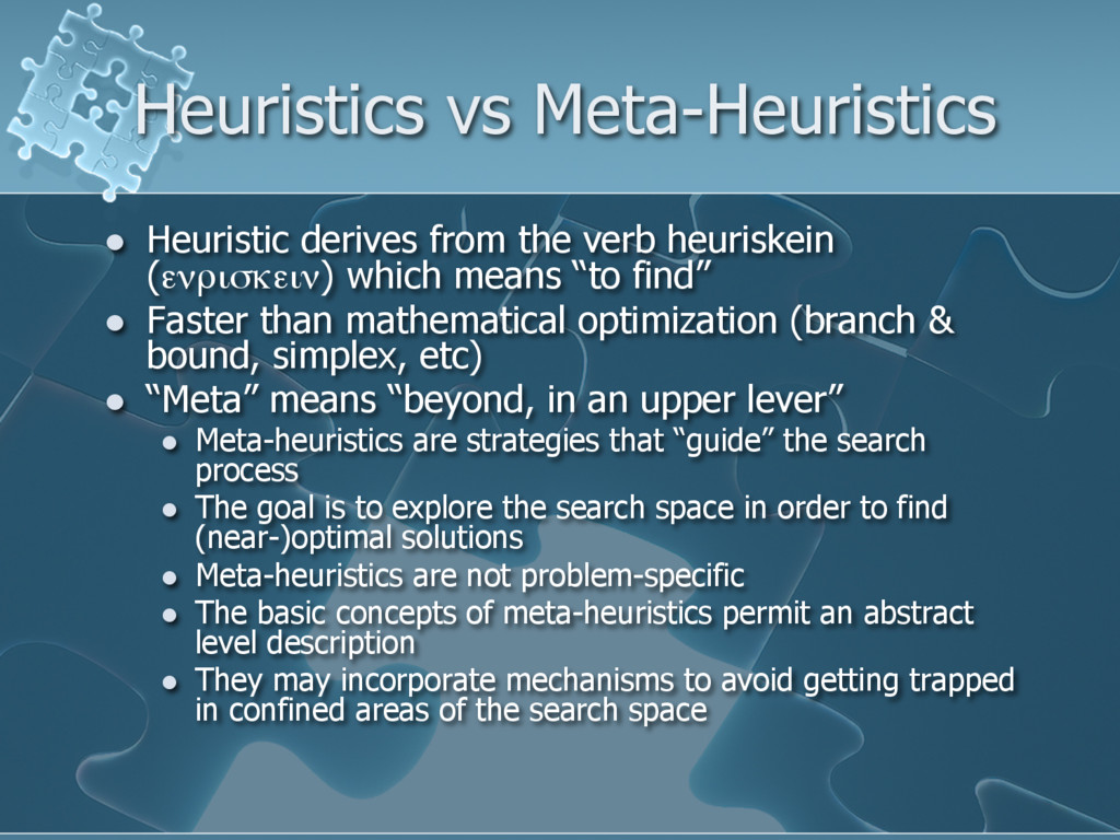
4. Heuristics vs Meta-Heuristics l  Heuristic derives from the verb heuriskein (ενρισκειν) which means “to find” l  Faster than mathematical optimization (branch & bound, simplex, etc) l  “Meta” means “beyond, in an upper lever” l  Meta-heuristics are strategies that “guide” the search process l  The goal is to explore the search space in order to find (near-)optimal solutions l  Meta-heuristics are not problem-specific l  The basic concepts of meta-heuristics permit an abstract level description l  They may incorporate mechanisms to avoid getting trapped in confined areas of the search space
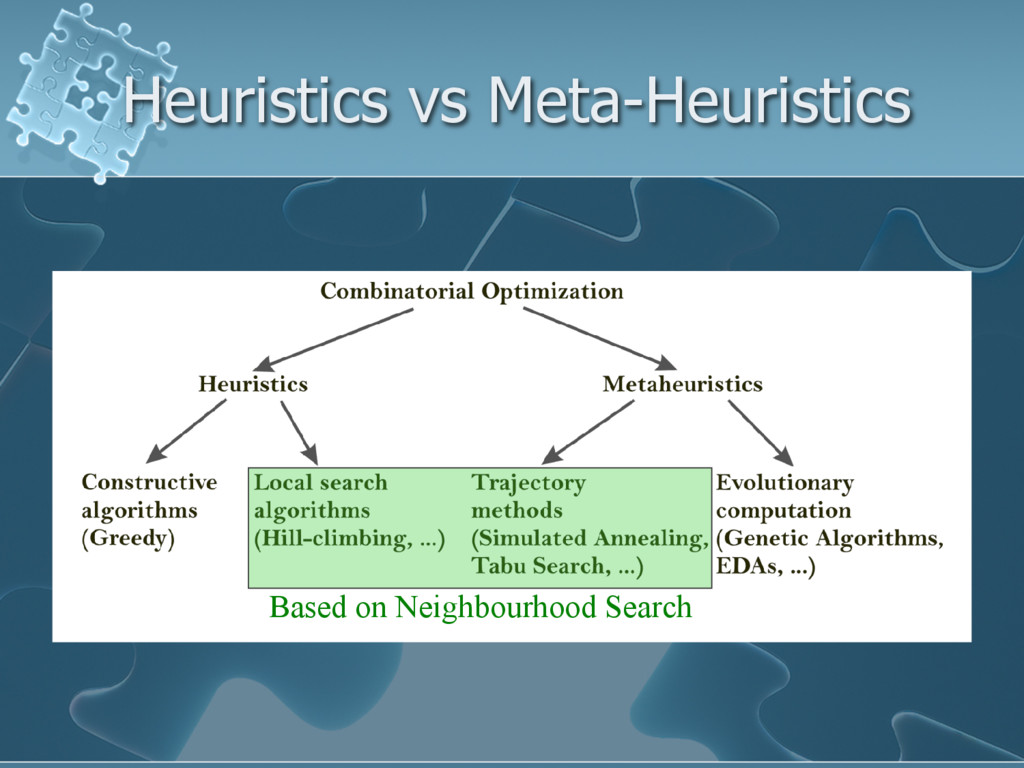
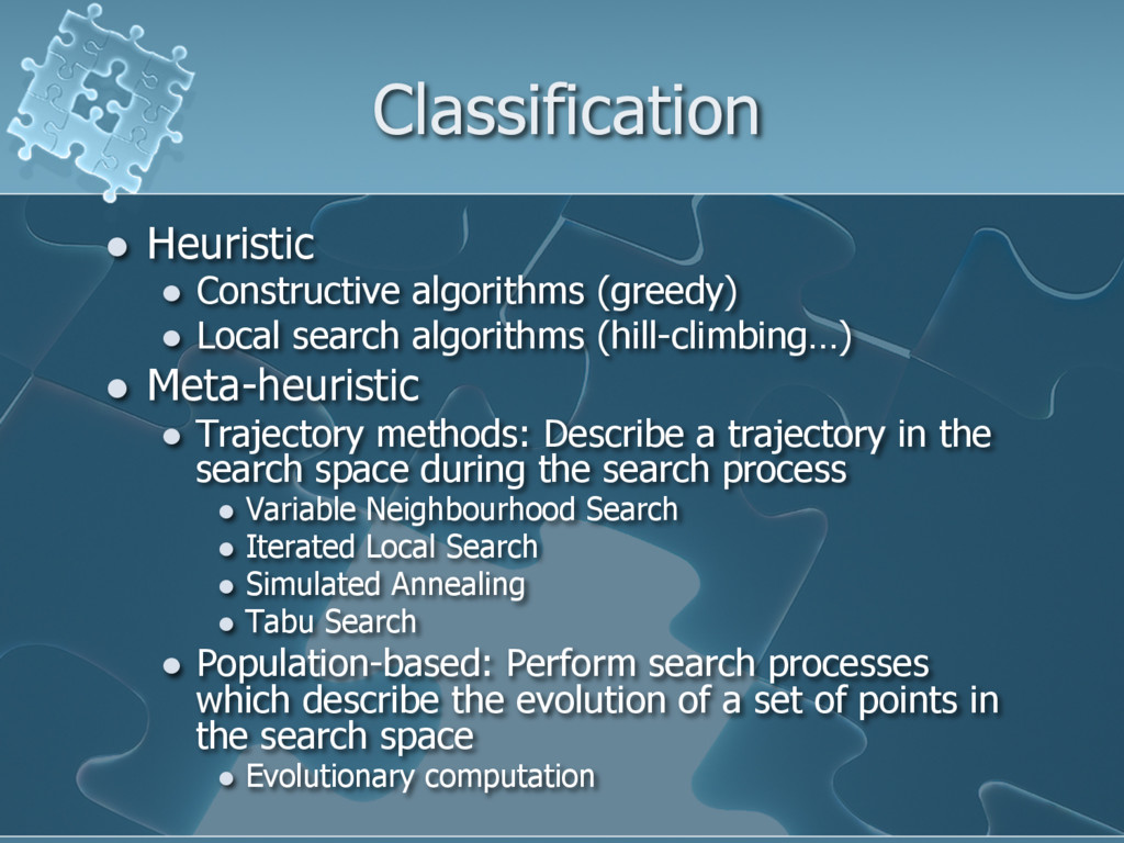
5. Classification l  Heuristic l  Constructive algorithms (greedy) l  Local search algorithms (hill-climbing…) l  Meta-heuristic l  Trajectory methods: Describe a trajectory in the search space during the search process l  Variable Neighbourhood Search l  Iterated Local Search l  Simulated Annealing l  Tabu Search l  Population-based: Perform search processes which describe the evolution of a set of points in the search space l  Evolutionary computation
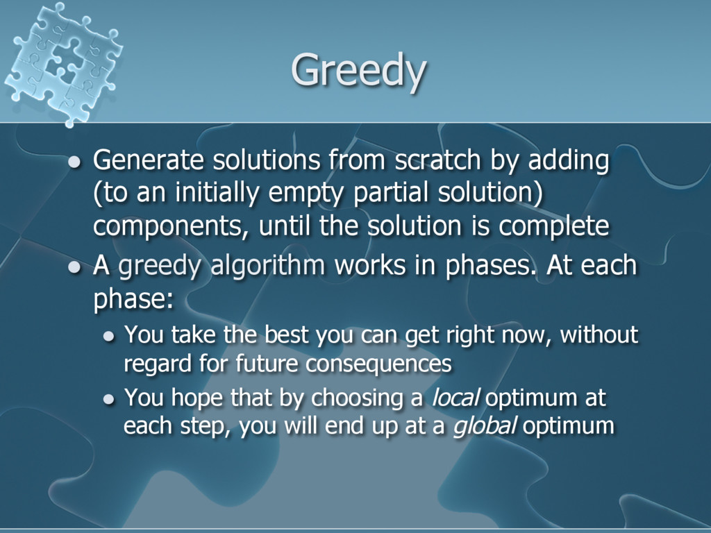
6. Greedy l  Generate solutions from scratch by adding (to an initially empty partial solution) components, until the solution is complete l  A greedy algorithm works in phases. At each phase: l  You take the best you can get right now, without regard for future consequences l  You hope that by choosing a local optimum at each step, you will end up at a global optimum
7. Greedy: Example l  Scheduling: l  3 processors l  9 jobs (3, 5, 6, 10, 11, 14, 15, 18 and 20 minutes) l  Greedy assign to each free processor the longest-running job 20 18 15 14 11 10 6 5 3 P1 P2 P3 Total time: 35 m
8. Greedy: Example l  Scheduling: l  3 processors l  9 jobs (3, 5, 6, 10, 11, 14, 15, 18 and 20 minutes) l  Greedy assign to each free processor the shortest-running job 20 18 15 14 11 10 6 5 3 P1 P2 P3 Total time: 40 m
9. Greedy: Example 20 18 15 14 11 10 6 5 3 P1 P2 P3 Longest-running job: 35 minutes 20 18 15 14 11 10 6 5 3 P1 P2 P3 Shortest-running job: 40 minutes 20 18 15 14 11 10 6 5 3 P1 P2 P3 Optimal: 34 minutes
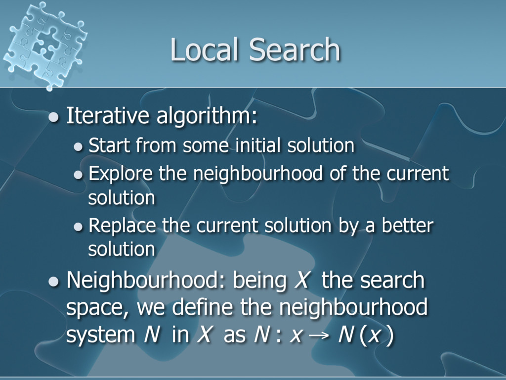
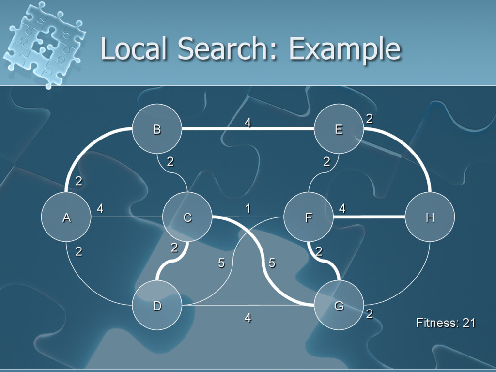
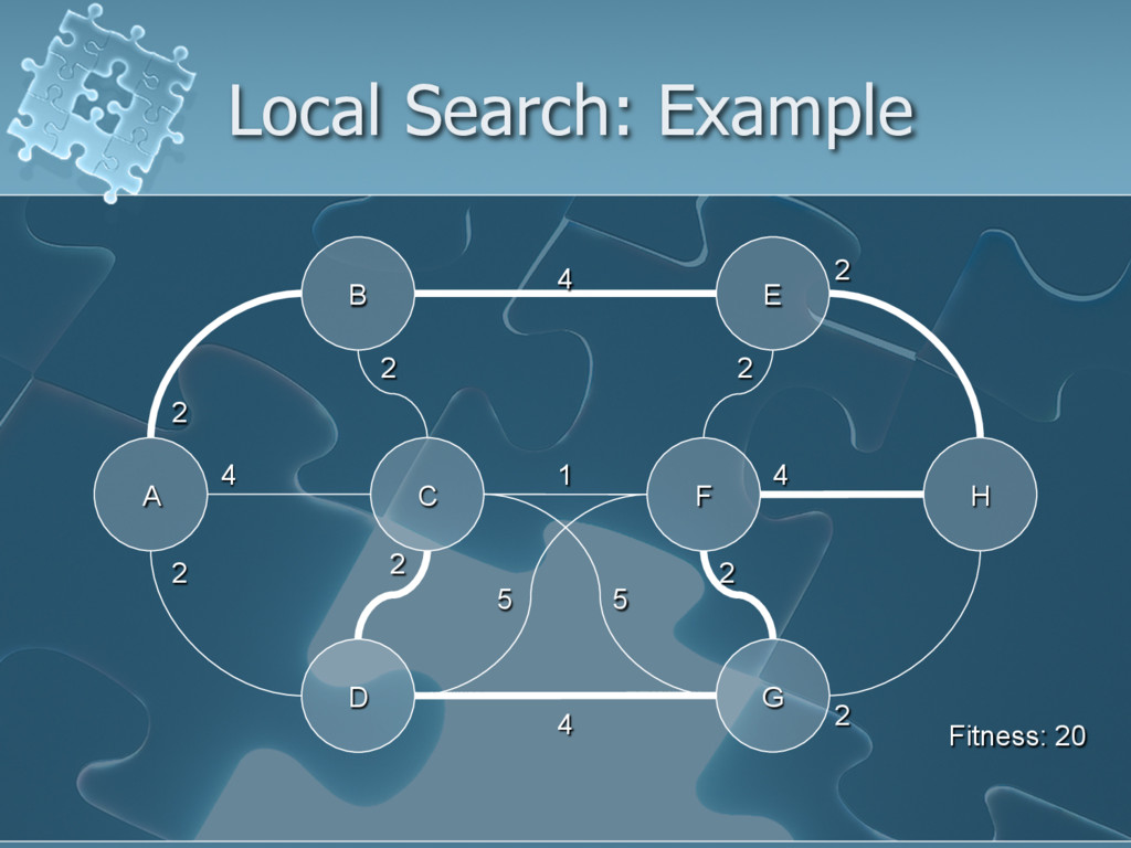
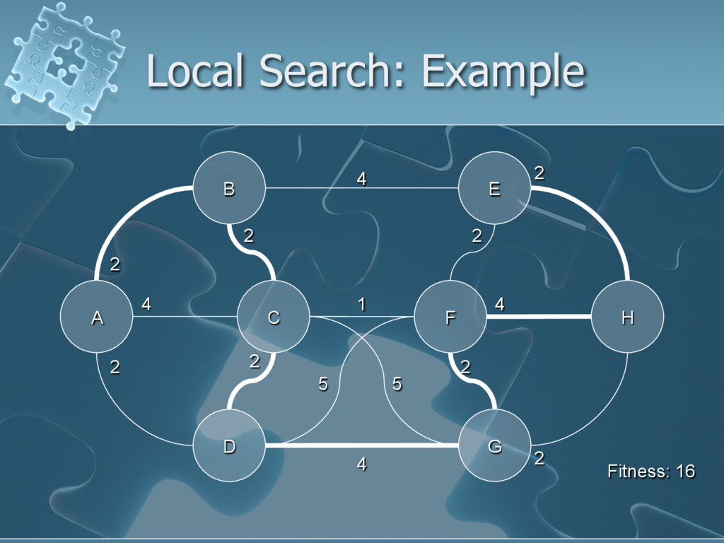
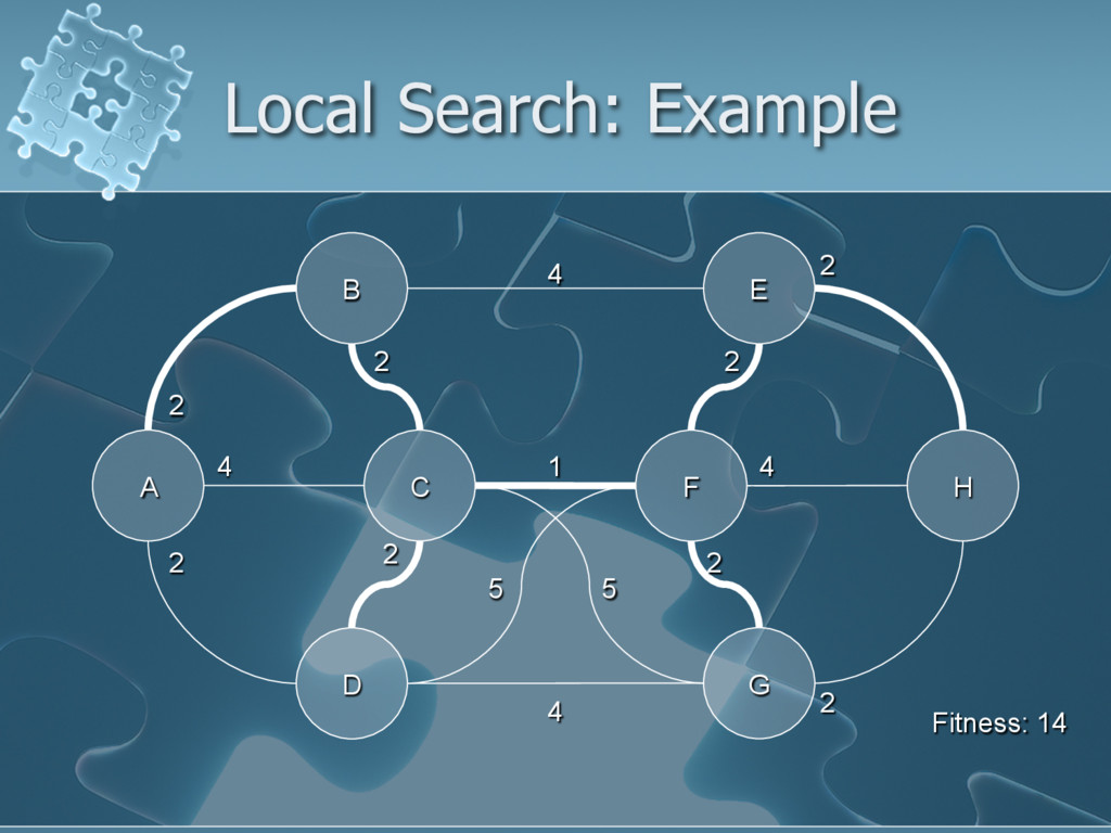
10. Local Search l  Iterative algorithm: l  Start from some initial solution l  Explore the neighbourhood of the current solution l  Replace the current solution by a better solution l  Neighbourhood: being X the search space, we define the neighbourhood system N in X as N : x → N (x )
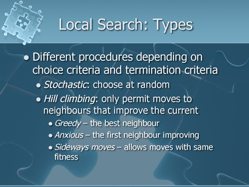
11. Local Search: Types l  Different procedures depending on choice criteria and termination criteria l  Stochastic: choose at random l  Hill climbing: only permit moves to neighbours that improve the current l Greedy – the best neighbour l Anxious – the first neighbour improving l Sideways moves – allows moves with same fitness
12. Local Search s=GenerateInitialSolution() while Termination criteria not met s’=PickAtRandom( N(x) ) If ( f(s’) < f(s) ) then s=s’ Endif end while
13. Local Search: Example D B G E A H C F 2 2 4 4 2 2 2 2 5 2 4 5 2 4 1
14. Local Search: Example D B G E A H C F 2 2 4 4 2 2 2 2 5 2 4 5 2 4 1 Fitness: 20
15. Local Search: Example D B G E A H C F 2 2 4 4 2 2 2 2 5 2 4 5 2 4 1 Fitness: 21
16. Local Search: Example D B G E A H C F 2 2 4 4 2 2 2 2 5 2 4 5 2 4 1 Fitness: 20
17. Local Search: Example D B G E A H C F 2 2 4 4 2 2 2 2 5 2 4 5 2 4 1 Fitness: 16
18. Local Search: Example D B G E A H C F 2 2 4 4 2 2 2 2 5 2 4 5 2 4 1 Fitness: 14
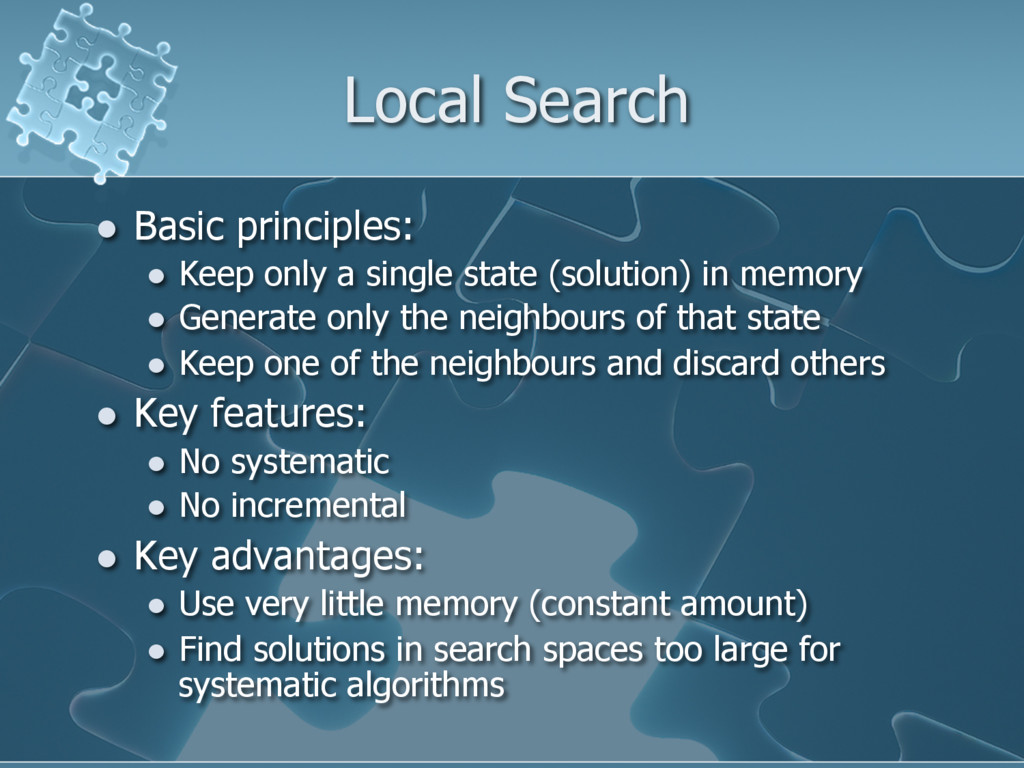
19. Local Search l  Basic principles: l  Keep only a single state (solution) in memory l  Generate only the neighbours of that state l  Keep one of the neighbours and discard others l  Key features: l  No systematic l  No incremental l  Key advantages: l  Use very little memory (constant amount) l  Find solutions in search spaces too large for systematic algorithms
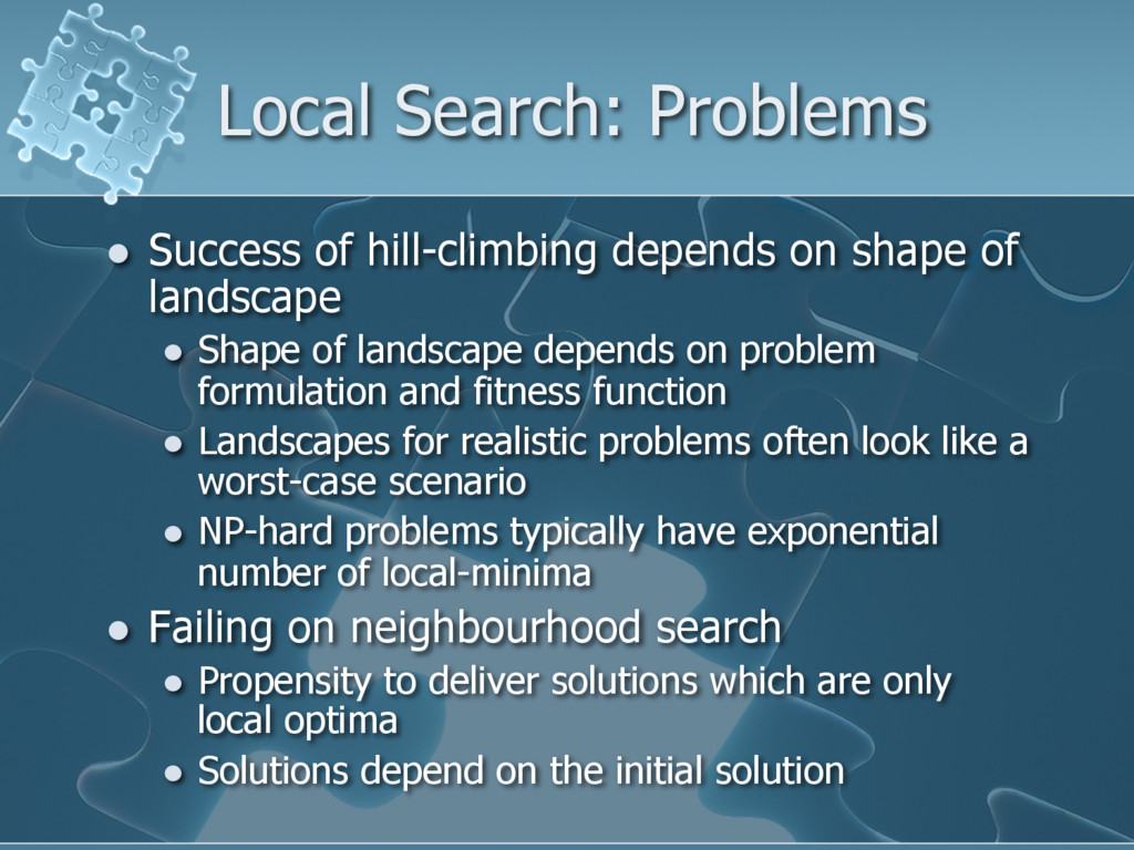
20. Local Search: Problems l  Success of hill-climbing depends on shape of landscape l  Shape of landscape depends on problem formulation and fitness function l  Landscapes for realistic problems often look like a worst-case scenario l  NP-hard problems typically have exponential number of local-minima l  Failing on neighbourhood search l  Propensity to deliver solutions which are only local optima l  Solutions depend on the initial solution
21. Local Search: Solutions l  Applies local search to an initial solution until it finds the local optimum; then it perturbs the solution and it restarts local search
22. Local Search: Solutions l  Strategy based on dynamically changing neighborhood structure
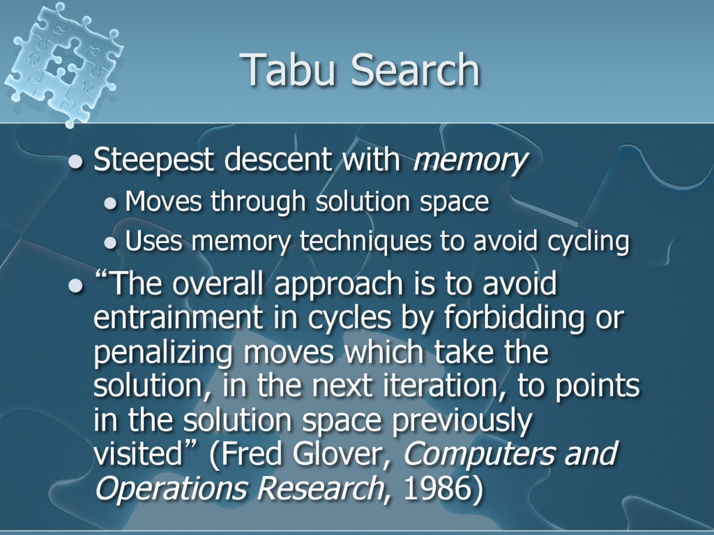
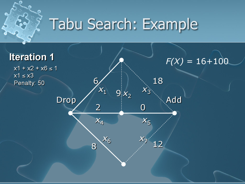
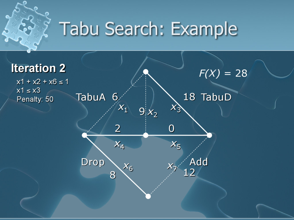
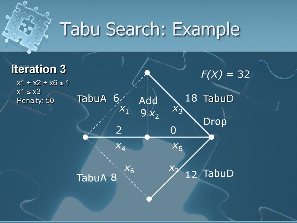
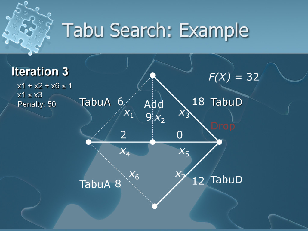
23. Tabu Search l  Steepest descent with memory l  Moves through solution space l  Uses memory techniques to avoid cycling l  “The overall approach is to avoid entrainment in cycles by forbidding or penalizing moves which take the solution, in the next iteration, to points in the solution space previously visited” (Fred Glover, Computers and Operations Research, 1986)
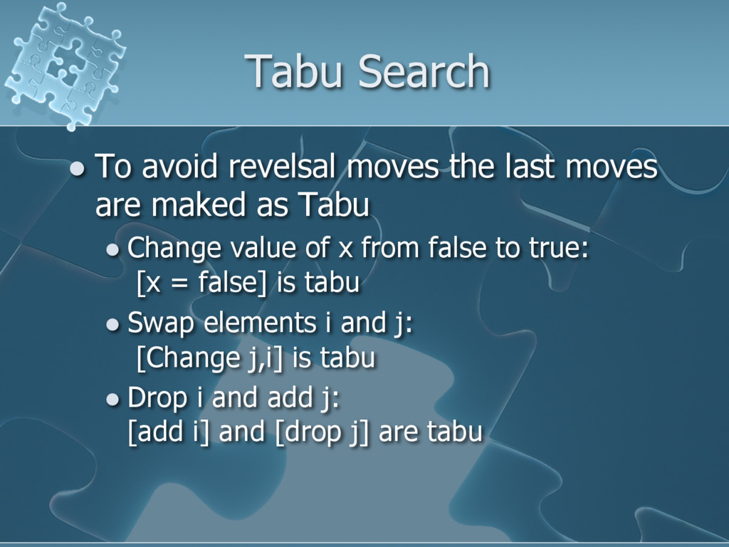
24. Tabu Search l  To avoid revelsal moves the last moves are maked as Tabu l  Change value of x from false to true: [x = false] is tabu l  Swap elements i and j: [Change j,i] is tabu l  Drop i and add j: [add i] and [drop j] are tabu
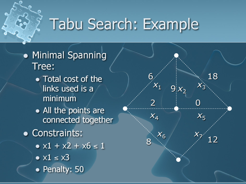
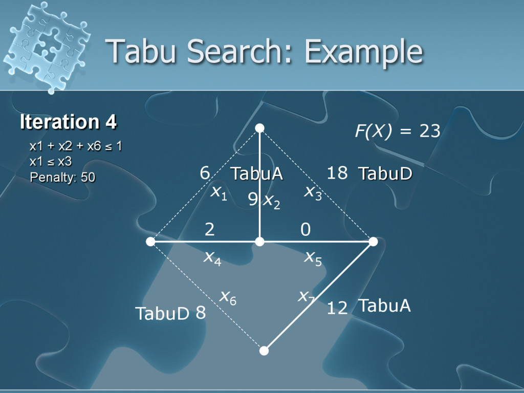
25. Tabu Search: Example l  Minimal Spanning Tree: l  Total cost of the links used is a minimum l  All the points are connected together l  Constraints: l  x1 + x2 + x6 ≤ 1 l  x1 ≤ x3 l  Penalty: 50 x1 x2 x3 x4 x6 x7 x5 6 2 0 8 12 18 9
26. Tabu Search: Example l  The move considered is the standard “edge swap” move l  An edge is listed as tabu l  if it was added within the last two iterations l  if it was deleted within the last two iterations
27. Tabu Search: Example x1 x2 x3 x4 x6 x7 x5 6 2 0 8 12 18 9 Add Drop x1 + x2 + x6 ≤ 1 x1 ≤ x3 Penalty: 50 Iteration 1 F(X) = 16+100
28. Tabu Search: Example x1 x2 x3 x4 x6 x7 x5 6 2 0 8 12 18 9 TabuA Add Drop Iteration 2 x1 + x2 + x6 ≤ 1 x1 ≤ x3 Penalty: 50 TabuD F(X) = 28
29. Tabu Search: Example x1 x2 x3 x4 x6 x7 x5 6 2 0 8 12 18 9 F(X) = 32 TabuA Drop Add Iteration 3 x1 + x2 + x6 ≤ 1 x1 ≤ x3 Penalty: 50 TabuA TabuD TabuD
30. Tabu Search: Example x1 x2 x3 x4 x6 x7 x5 6 2 0 8 12 18 9 F(X) = 32 TabuA Drop Add Iteration 3 x1 + x2 + x6 ≤ 1 x1 ≤ x3 Penalty: 50 TabuA TabuD TabuD
31. Tabu Search: Example x1 x2 x3 x4 x6 x7 x5 6 2 0 8 12 18 9 Iteration 4 x1 + x2 + x6 ≤ 1 x1 ≤ x3 Penalty: 50 TabuD TabuA TabuD TabuA F(X) = 23
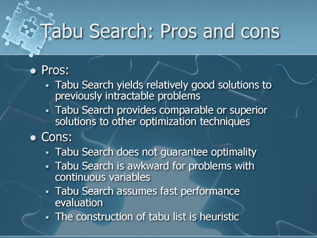
32. Tabu Search: Pros and cons l  Pros: §  Tabu Search yields relatively good solutions to previously intractable problems §  Tabu Search provides comparable or superior solutions to other optimization techniques l  Cons: §  Tabu Search does not guarantee optimality §  Tabu Search is awkward for problems with continuous variables §  Tabu Search assumes fast performance evaluation §  The construction of tabu list is heuristic
33. Simulated Annealing l  Based on the cooling of material in a heat bath l  Local Search but we allow moves resulting in solutions of worse quality than the current solution l  Avoid from local solutions
34. Simulated Annealing
35. Simulated Annealing s=GenerateInitialSolution() t=t(0) while Termination criteria not met s’=PickAtRandom( N(x) ) If ( f(s’) < f(s) ) then s=s’ else Accept s’ as new solution with probability Endif Update(T) end while ( ') ( ) f s f s T e − −
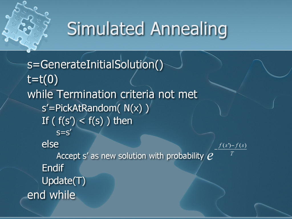
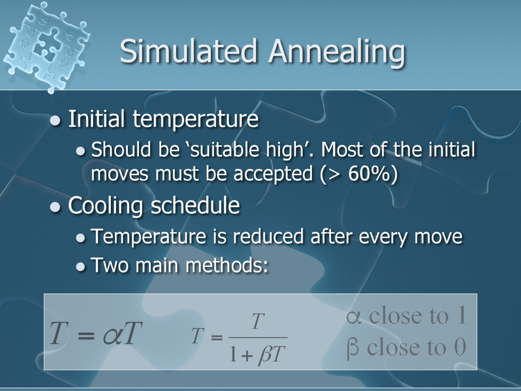
36. Simulated Annealing l  Initial temperature l  Should be ‘suitable high’. Most of the initial moves must be accepted (> 60%) l  Cooling schedule l  Temperature is reduced after every move l  Two main methods: T T α = T T T β + = 1 α close to 1 β close to 0