OpenTalks.AI - Евгений Бурнаев, Байесовская фильтрация в латентном пространстве для прогнозирования чистого дохода Банка от эквайринга

Transcript

1. 1/27 Bayesian Models for Prediction of Deposit Churn Profile and Net Income from Acquiring Sberbank, Treasury Sergey Strelkov, Ksenia Gubina, Denis Orlov Skoltech, ADASE Evgeny Burnaev, Evgeny Egorov
2. 2/27 Macro-data Banking performance depends on the macroeconomic situation, characterized by interbank foreign exchange rates, etc. Ruble interbank rates
3. 3/27 Macro-data Vertical lines moments of significant Deposits Сhurn Currency interbank rates vs. time
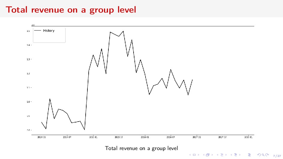
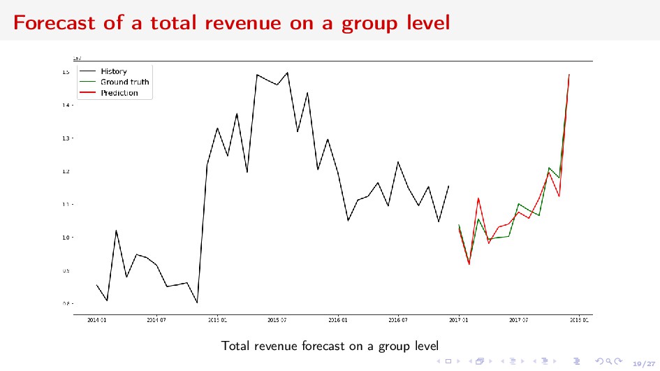
4. 4/27 Prediction of Deposits Churn and Income from Acquiring Capital adequacy and liquidity risks ⇒ long-term forecasting Deposits Churn Net Revenue from Acquiring Vintage economic units grouped by some categorical characteristics and united by time interval Forecast the value of the vintage, or the sum w.r.t. some vintages
5. 5/27 Acquiring 48 groups j (segment, territory, affiliation of a client to a bank) Vintage w.r.t. to a starting month of a contract Forecast: for each group j total (w.r.t. vintages) Net Revenue 12 months ahead (yt+1 j , . . . , yt+12 j ) Code num Segment Terbank Client Num. of Vintages 0 Client CIB Baykal bank NON-SB 131 . . . . . . . . . . . . . . . 47 Client of the block “Corp. business” South-West bank SB 182 Accuracy Metric: L(y, ˆ y) = j∈CodeNum yj − ˆ yj 1 yj 1
6. 6/27 Revenue on a vintage level Revenue for a single vintage
7. 7/27 Total revenue on a group level Total revenue on a group level
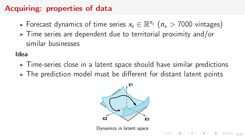
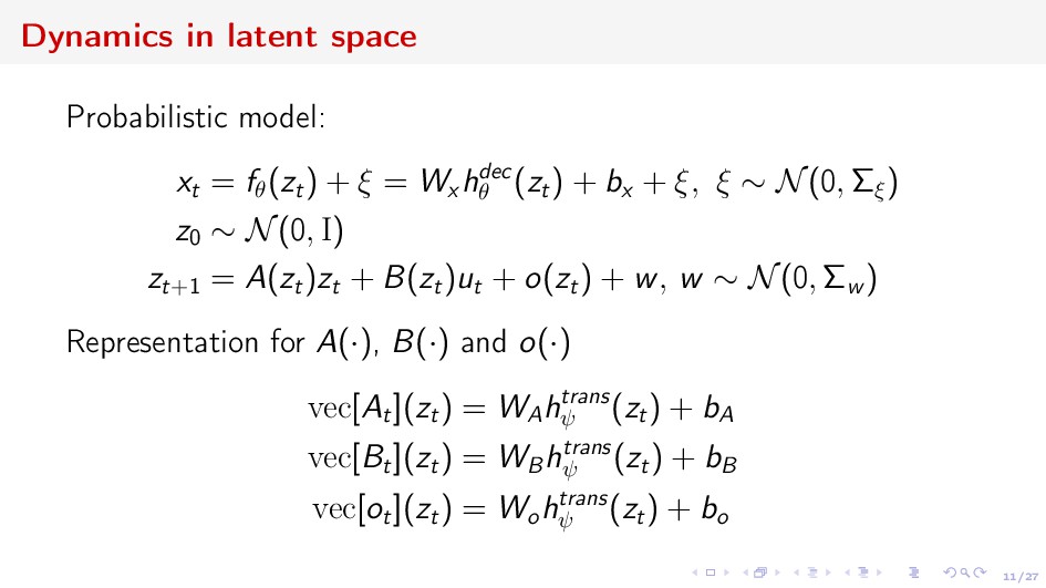
8. 8/27 Acquiring: properties of data Forecast dynamics of time series xt ∈ Rnx (nx > 7000 vintages) Time series are dependent due to territorial proximity and/or similar businesses Idea Time-series close in a latent space should have similar predictions The prediction model must be different for distant latent points Dynamics in latent space
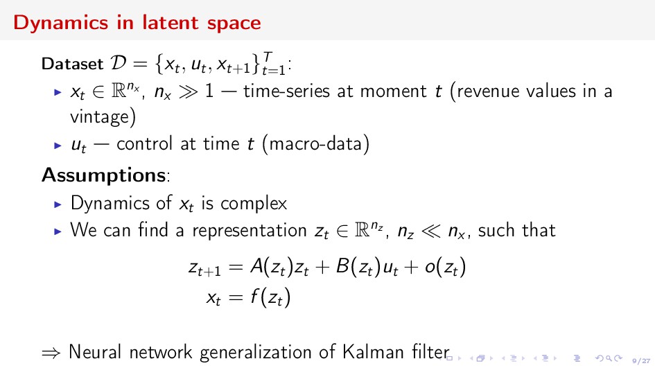
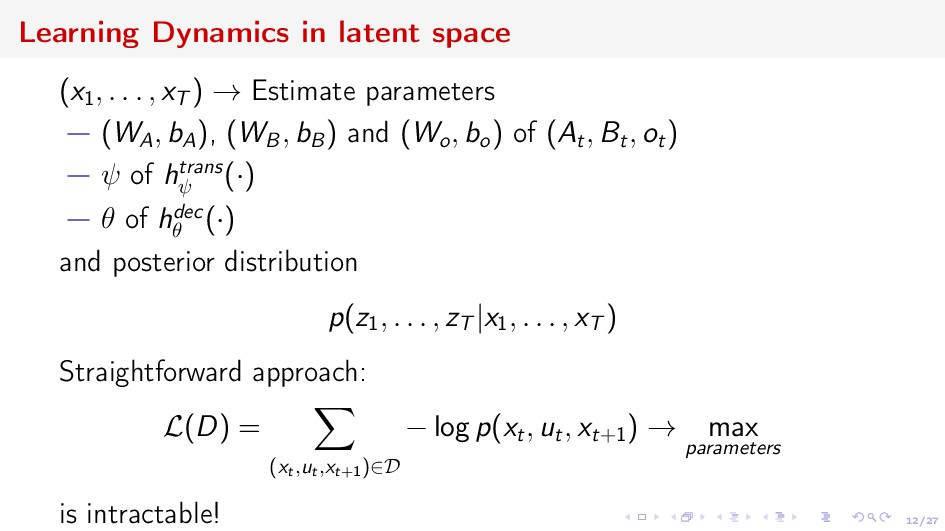
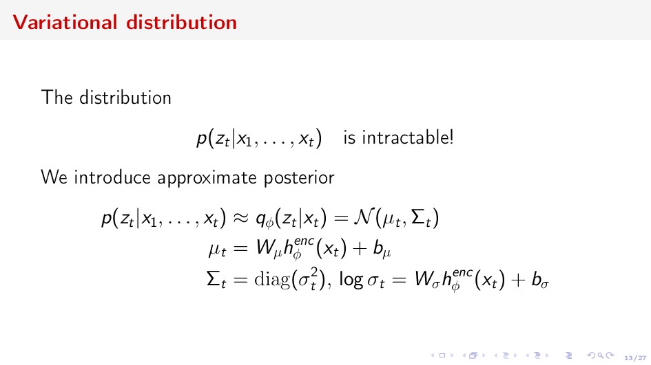
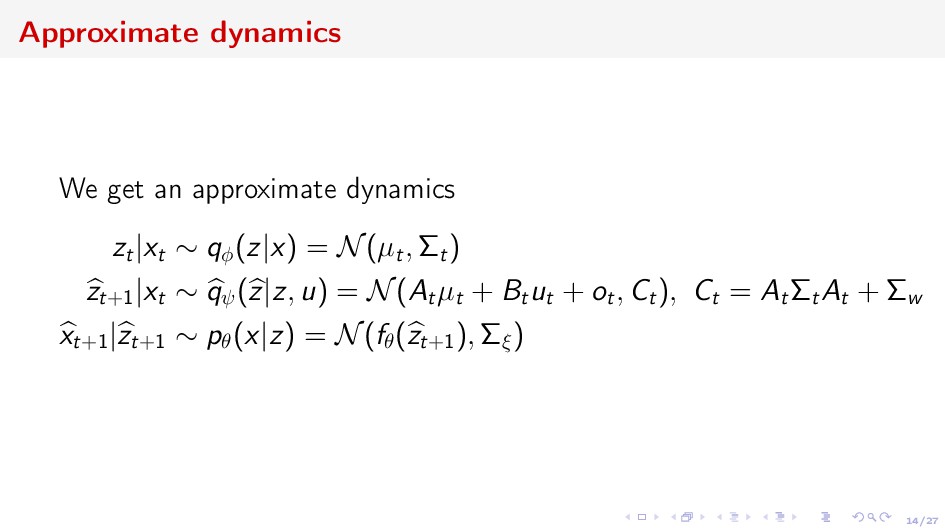
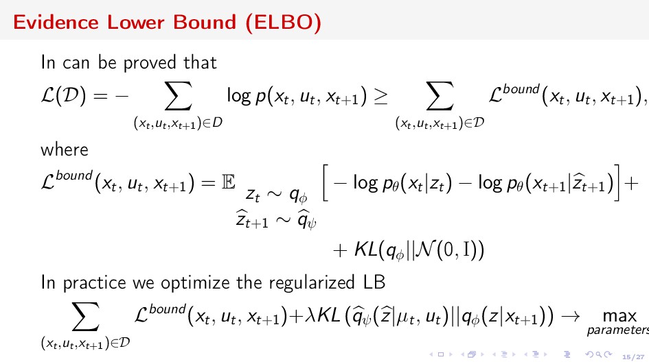
9. 9/27 Dynamics in latent space Dataset D = {xt , ut , xt+1 }T t=1 : xt ∈ Rnx , nx 1 time-series at moment t (revenue values in a vintage) ut control at time t (macro-data) Assumptions: Dynamics of xt is complex We can find a representation zt ∈ Rnz , nz nx , such that zt+1 = A(zt )zt + B(zt )ut + o(zt ) xt = f (zt ) ⇒ Neural network generalization of Kalman filter
10. 10/27 Example of a Neural Network: Equations Universal mapping x → y = hθ (x) a(j) i = – “activation” θ(j) = – weight matrix Typically g(x) = max(x, 0) a(2) 1 = g θ(1) 10 x0 + θ(1) 11 x1 + θ(1) 12 x2 + θ(1) 13 x3 a(2) 2 = g θ(1) 20 x0 + θ(1) 21 x1 + θ(1) 22 x2 + θ(1) 23 x3 a(2) 3 = g θ(1) 30 x0 + θ(1) 31 x1 + θ(1) 32 x2 + θ(1) 33 x3 hθ (x) = a(3) 1 = θ(2) 10 a(2) 0 + θ(2) 11 a(2) 1 + θ(2) 12 a(2) 2 + θ(2) 13 a(2) 3
11. 11/27 Dynamics in latent space Probabilistic model: xt = fθ (zt ) + ξ = Wx hdec θ (zt ) + bx + ξ, ξ ∼ N(0, Σξ ) z0 ∼ N(0, I) zt+1 = A(zt )zt + B(zt )ut + o(zt ) + w, w ∼ N(0, Σw ) Representation for A(·), B(·) and o(·) vec[At ](zt ) = WA htrans ψ (zt ) + bA vec[Bt ](zt ) = WB htrans ψ (zt ) + bB vec[ot ](zt ) = Wo htrans ψ (zt ) + bo
12. 12/27 Learning Dynamics in latent space (x1 , . . . , xT ) → Estimate parameters (WA , bA ), (WB , bB ) and (Wo , bo ) of (At , Bt , ot ) ψ of htrans ψ (·) θ of hdec θ (·) and posterior distribution p(z1 , . . . , zT |x1 , . . . , xT ) Straightforward approach: L(D) = (xt,ut,xt+1 )∈D − log p(xt , ut , xt+1 ) → max parameters is intractable!
13. 13/27 Variational distribution The distribution p(zt |x1 , . . . , xt ) is intractable! We introduce approximate posterior p(zt |x1 , . . . , xt ) ≈ qφ (zt |xt ) = N(µt , Σt ) µt = Wµ henc φ (xt ) + bµ Σt = diag(σ2 t ), log σt = Wσ henc φ (xt ) + bσ
14. 14/27 Approximate dynamics We get an approximate dynamics zt |xt ∼ qφ (z|x) = N(µt , Σt ) zt+1 |xt ∼ qψ (z|z, u) = N(At µt + Bt ut + ot , Ct ), Ct = At Σt At + Σw xt+1 |zt+1 ∼ pθ (x|z) = N(fθ (zt+1 ), Σξ )
15. 15/27 Evidence Lower Bound (ELBO) In can be proved that L(D) = − (xt,ut,xt+1 )∈D log p(xt , ut , xt+1 ) ≥ (xt,ut,xt+1 )∈D Lbound(xt , ut , xt+1 ), where Lbound(xt , ut , xt+1 ) = E zt ∼ qφ zt+1 ∼ qψ − log pθ (xt |zt ) − log pθ (xt+1 |zt+1 ) + + KL(qφ ||N(0, I)) In practice we optimize the regularized LB (xt,ut,xt+1 )∈D Lbound(xt , ut , xt+1 )+λKL (qψ (z|µt , ut )||qφ (z|xt+1 )) → max parameters
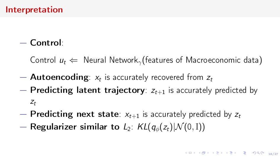
16. 16/27 Interpretation Control: Control ut ⇐ Neural Networkγ (features of Macroeconomic data) Autoencoding: xt is accurately recovered from zt Predicting latent trajectory: zt+1 is accurately predicted by zt Predicting next state: xt+1 is accurately predicted by zt Regularizer similar to L2 : KL(qφ (zt )|N(0, I))
17. 17/27 Forecast on a vintage level Revenue forecast for a single vintage
18. 18/27 Forecast on a vintage level Revenue forecast for a single vintage
19. 19/27 Forecast of a total revenue on a group level Total revenue forecast on a group level
20. 20/27 Deposits Churn Fixed-term deposits of individuals on a level of vintages Vintage j deposits with the same charac-s (vintage code): Date of opening of a Deposit Deposit currency, term of Deposit Segment of a deposit, sales channel, volume, type of a deposit Has a deposit been prolonged? Forecast monthly change in a volume of a vintage (churn rate) EARt j = V t j − V t−1 j V t−1 j ∈ [−1; 0] In total 103932 vintages, and we have only 48 time points
21. 21/27 Deposits churn: problem statement Without observing vintage dynamics for a whole length of a deposit (3 − 18 months) predict: EARt=1,...,18 months = Predict(features of Macro, interest rates, etc.)
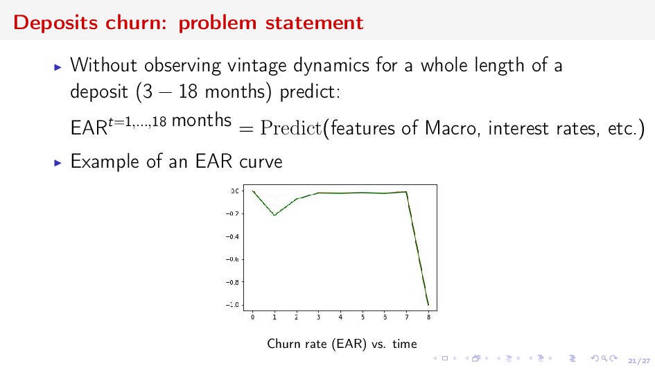
22. 21/27 Deposits churn: problem statement Without observing vintage dynamics for a whole length of a deposit (3 − 18 months) predict: EARt=1,...,18 months = Predict(features of Macro, interest rates, etc.) Example of an EAR curve Churn rate (EAR) vs. time
23. 22/27 Deposits churn: problem statement Performance: inequalities w.r.t. to net volumes V T i=1 j∈VintSet V i j − ˆ V i j 1 ≤ T i=1 V 0 j − ˆ V i j 1 T i=1 j∈VintSet V i j − ˆ V i j 1 ≤ T i=1 V 0 j − V i j 1
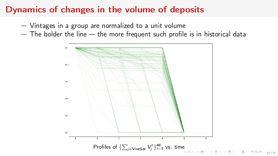
24. 23/27 Dynamics of changes in the volume of deposits Vintages in a group are normalized to a unit volume The bolder the line the more frequent such profile is in historical data Profiles of { j∈VintSet V t j }48 t=1 vs. time
25. 24/27 Multi-output GP f (·) ∼ GP( · |µ(z), K(z, z )) Features X features from macro-data ’RUBMP1’, ’USDLibor1’, ... (log-returns, variances, etc.) features from interest rates
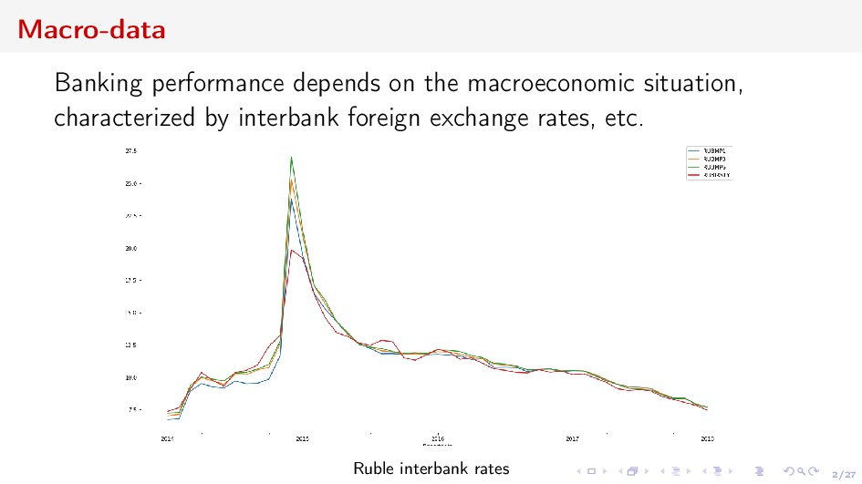
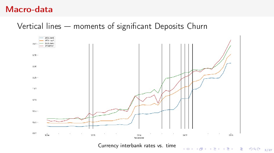
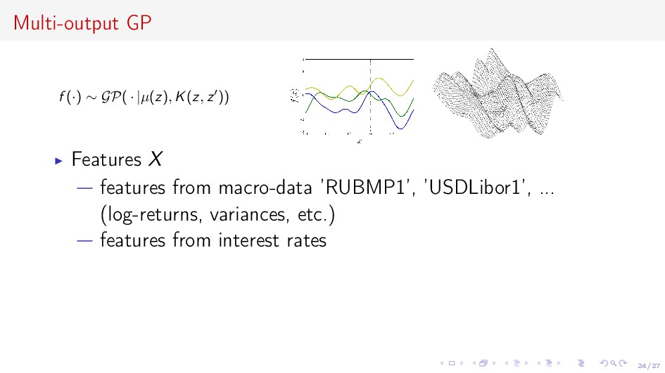
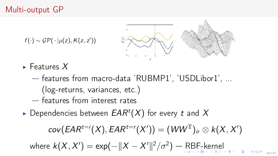
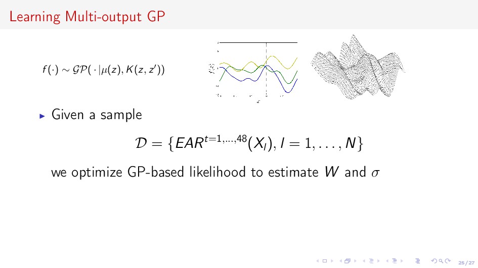
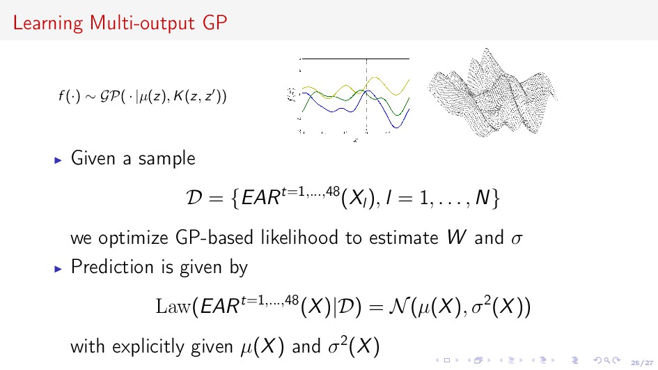
26. 24/27 Multi-output GP f (·) ∼ GP( · |µ(z), K(z, z )) Features X features from macro-data ’RUBMP1’, ’USDLibor1’, ... (log-returns, variances, etc.) features from interest rates Dependencies between EARt(X) for every t and X cov(EARt=i(X), EARt=r (X )) = (WW T)ir ⊗ k(X, X ) where k(X, X ) = exp(− X − X 2/σ2) RBF-kernel
27. 25/27 Learning Multi-output GP f (·) ∼ GP( · |µ(z), K(z, z )) Given a sample D = {EARt=1,...,48(Xl ), l = 1, . . . , N} we optimize GP-based likelihood to estimate W and σ
28. 25/27 Learning Multi-output GP f (·) ∼ GP( · |µ(z), K(z, z )) Given a sample D = {EARt=1,...,48(Xl ), l = 1, . . . , N} we optimize GP-based likelihood to estimate W and σ Prediction is given by Law(EARt=1,...,48(X)|D) = N(µ(X), σ2(X)) with explicitly given µ(X) and σ2(X)
29. 26/27 Results Inequalities for all codes, required by the customer better than results of XGBoost with some feature engineering Example of forecasts: (a) (b) Forecast of churn rates (EAR)
30. 27/27 Conclusions Modern Bayesian structural models R&D results are being tested Production implementation of the constructed models is planned