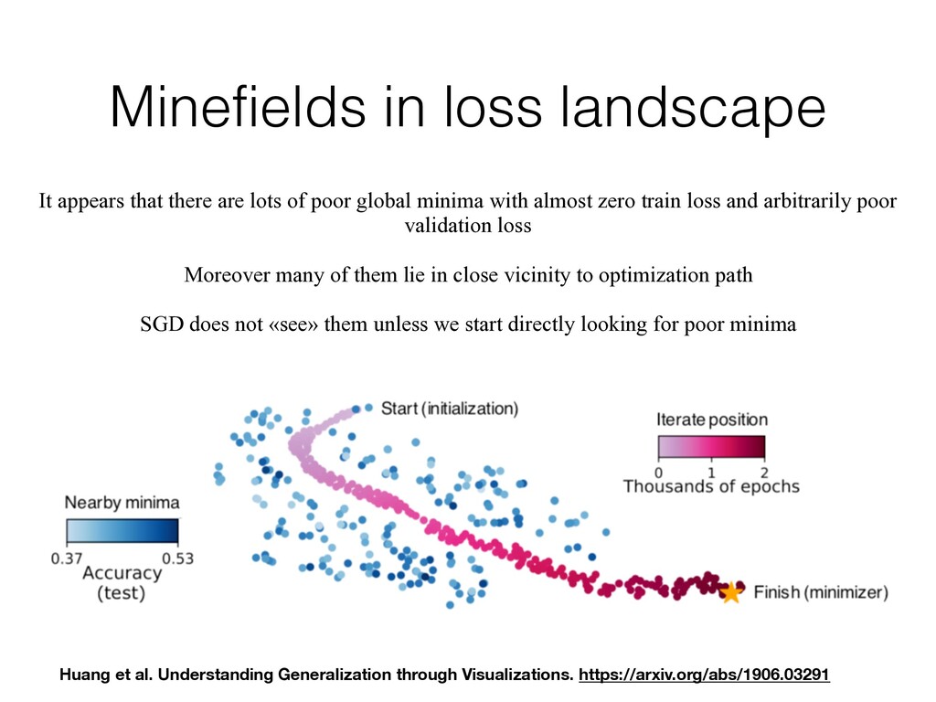
of poor global minima with almost zero train loss and arbitrarily poor validation loss Moreover many of them lie in close vicinity to optimization path SGD does not «see» them unless we start directly looking for poor minima Huang et al. Understanding Generalization through Visualizations. https://arxiv.org/abs/1906.03291
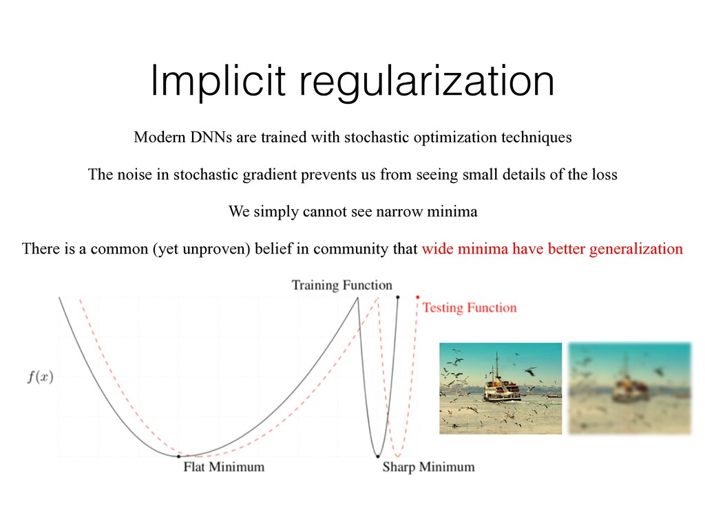
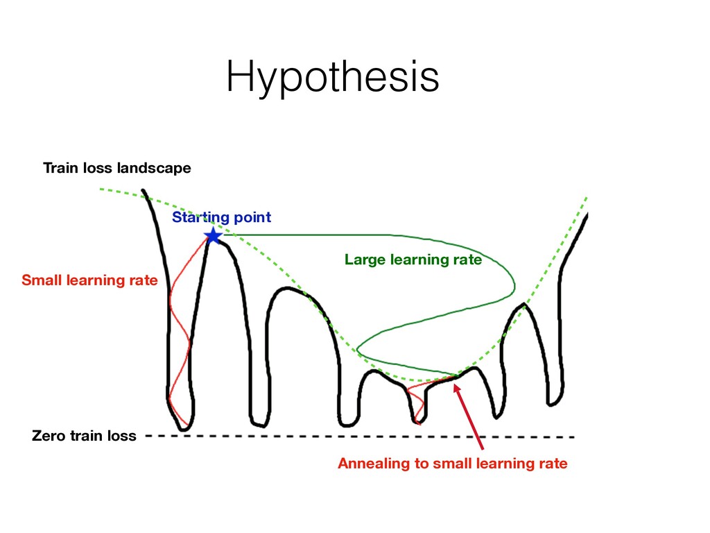
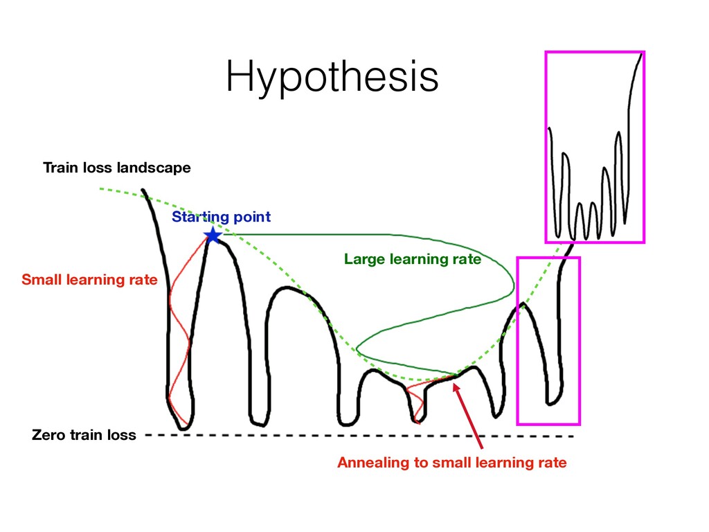
The noise in stochastic gradient prevents us from seeing small details of the loss We simply cannot see narrow minima There is a common (yet unproven) belief in community that wide minima have better generalization
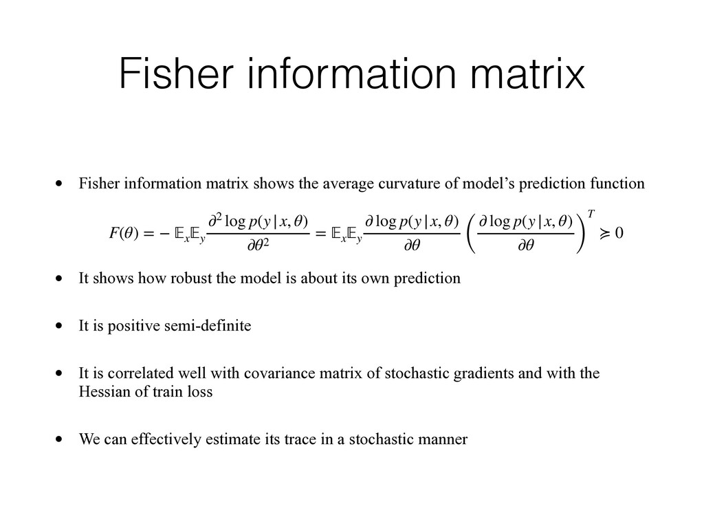
curvature of model’s prediction function • It shows how robust the model is about its own prediction • It is positive semi-definite • It is correlated well with covariance matrix of stochastic gradients and with the Hessian of train loss • We can effectively estimate its trace in a stochastic manner F(θ) = − 𝔼x 𝔼y ∂2 log p(y|x, θ) ∂θ2 = 𝔼x 𝔼y ∂ log p(y|x, θ) ∂θ ( ∂ log p(y|x, θ) ∂θ ) T ≽ 0
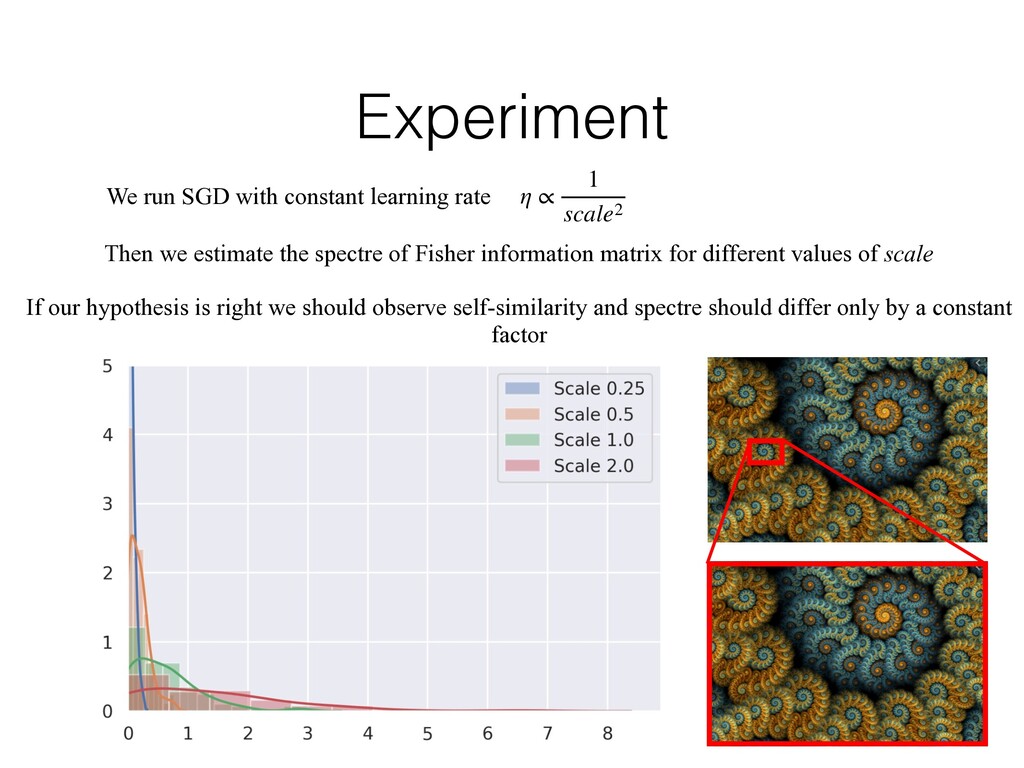
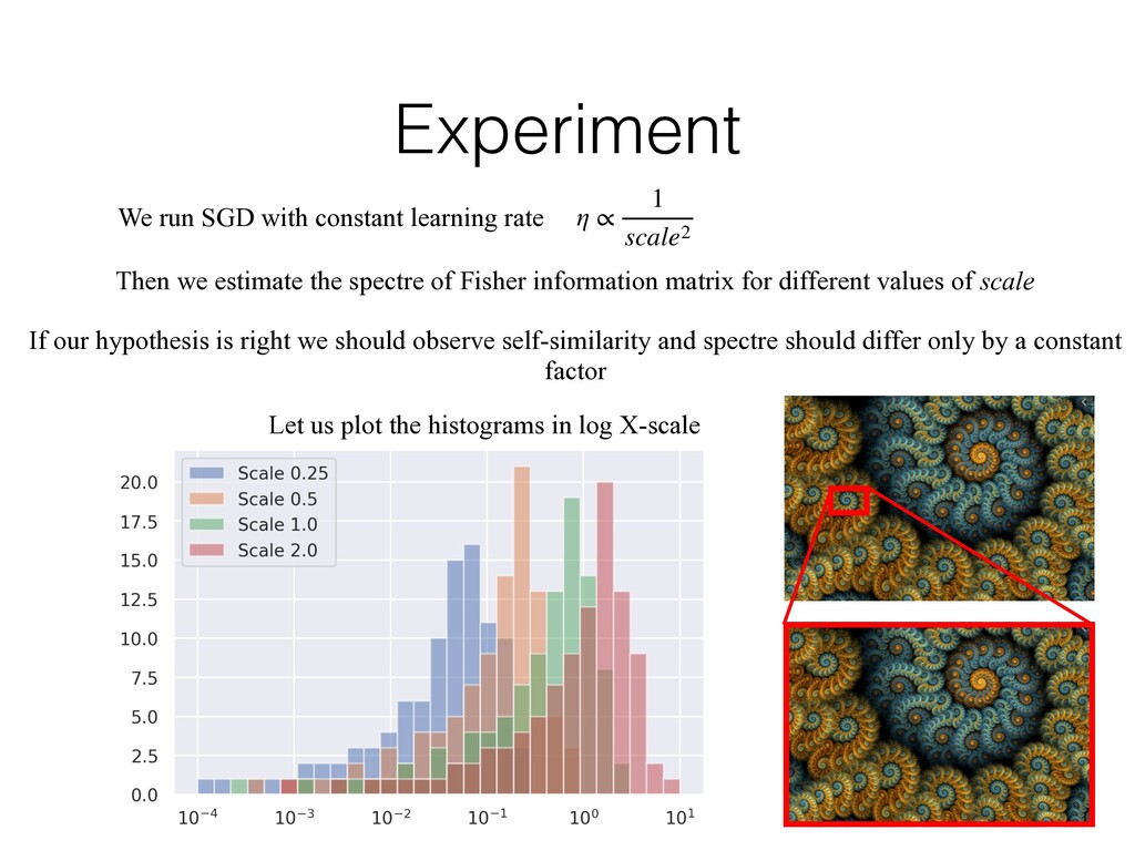
1 scale2 Then we estimate the spectre of Fisher information matrix for different values of scale If our hypothesis is right we should observe self-similarity and spectre should differ only by a constant factor
1 scale2 Then we estimate the spectre of Fisher information matrix for different values of scale If our hypothesis is right we should observe self-similarity and spectre should differ only by a constant factor Let us plot the histograms in log X-scale
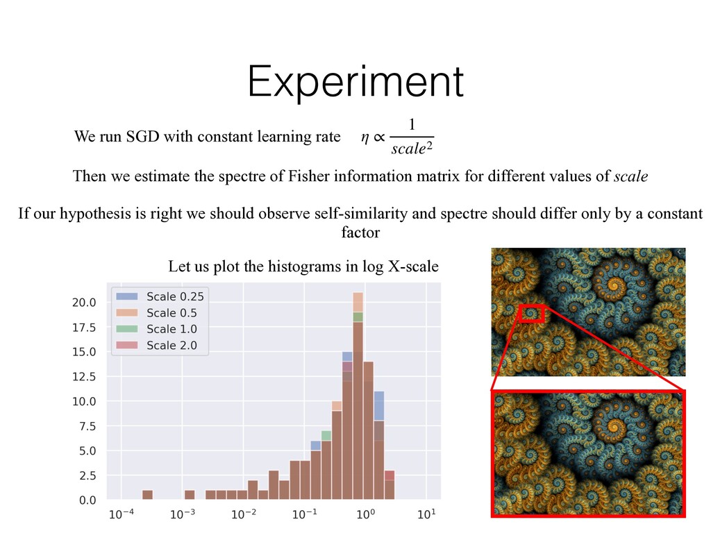
1 scale2 Then we estimate the spectre of Fisher information matrix for different values of scale If our hypothesis is right we should observe self-similarity and spectre should differ only by a constant factor Let us plot the histograms in log X-scale
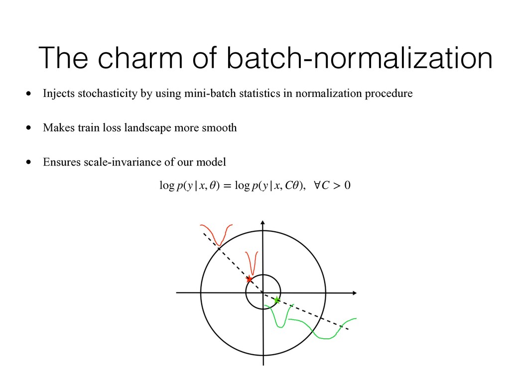
statistics in normalization procedure • Makes train loss landscape more smooth • Ensures scale-invariance of our model log p(y|x, θ) = log p(y|x, Cθ), ∀C > 0
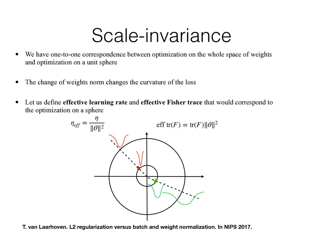
whole space of weights and optimization on a unit sphere • The change of weights norm changes the curvature of the loss • Let us define effective learning rate and effective Fisher trace that would correspond to the optimization on a sphere ηeff = η ∥θ∥2 eff tr(F) = tr(F)∥θ∥2 T. van Laarhoven. L2 regularization versus batch and weight normalization. In NIPS 2017.
training data is always orthogonal to the beam which connects the origin with the current weights • The gradient from weight decay is directed to the origin • The relation between data gradient and weight decay defines the change of the weights norm R. Wan, et al. Spherical motion dynamics: Learning dynamics of neural network with normalization, weight decay and SGD. https://arxiv.org/pdf/2006.08419.pdf
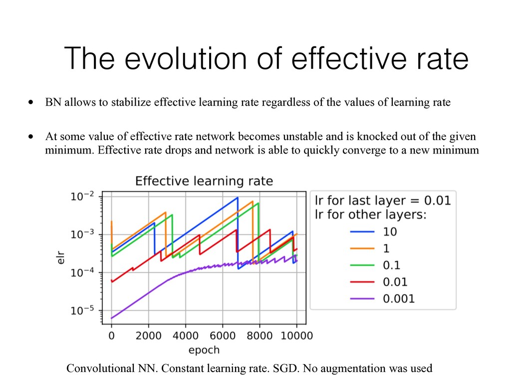
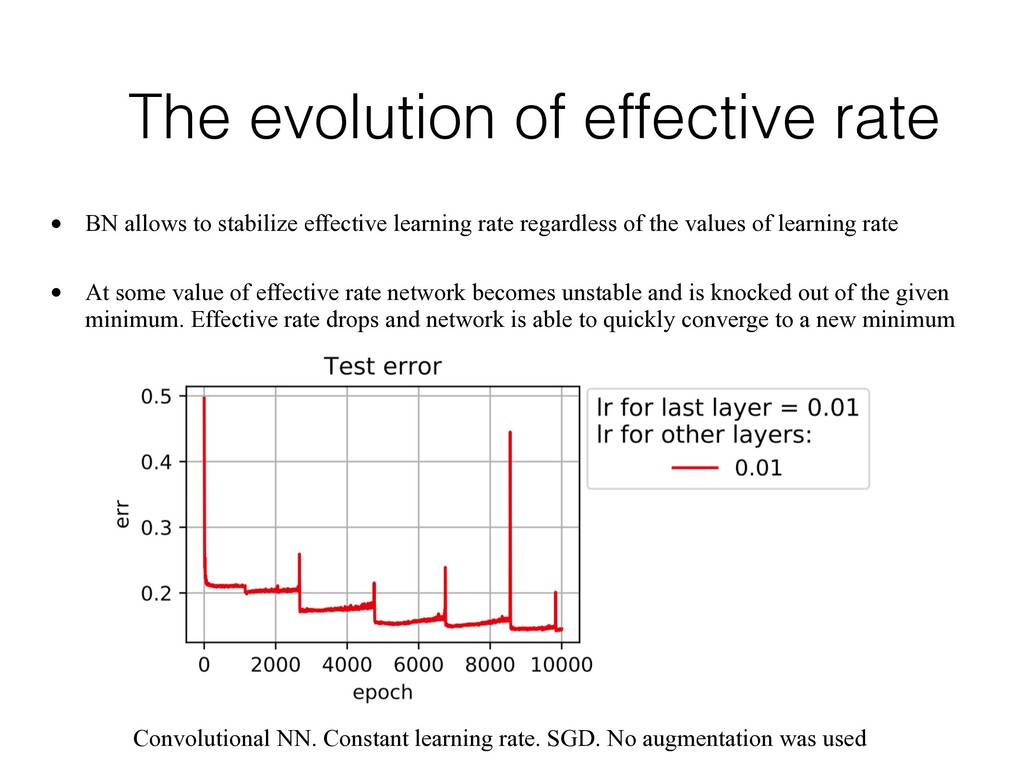
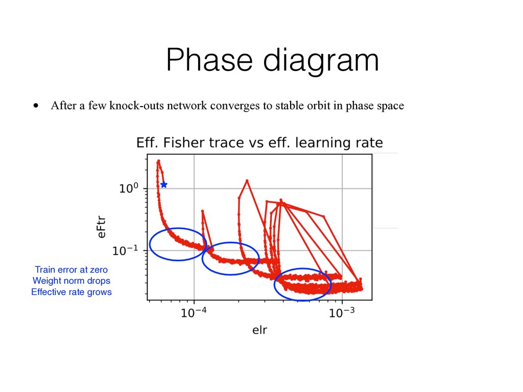
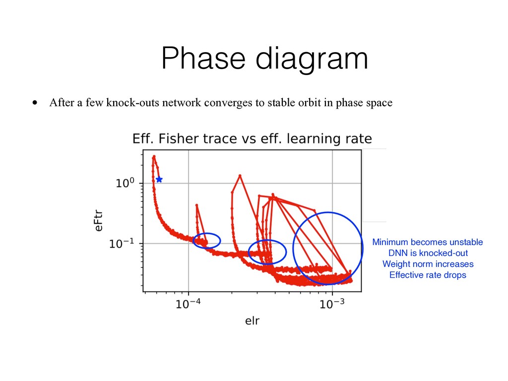
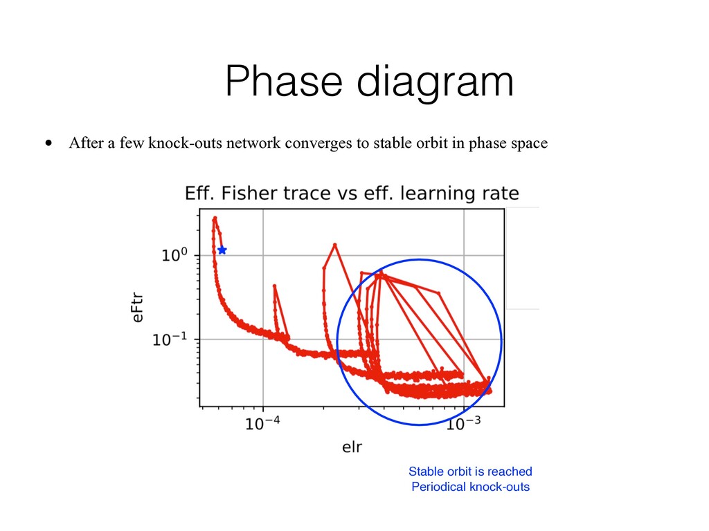
effective learning rate regardless of the values of learning rate • At some value of effective rate network becomes unstable and is knocked out of the given minimum. Effective rate drops and network is able to quickly converge to a new minimum Convolutional NN. Constant learning rate. SGD. No augmentation was used
effective learning rate regardless of the values of learning rate • At some value of effective rate network becomes unstable and is knocked out of the given minimum. Effective rate drops and network is able to quickly converge to a new minimum Convolutional NN. Constant learning rate. SGD. No augmentation was used
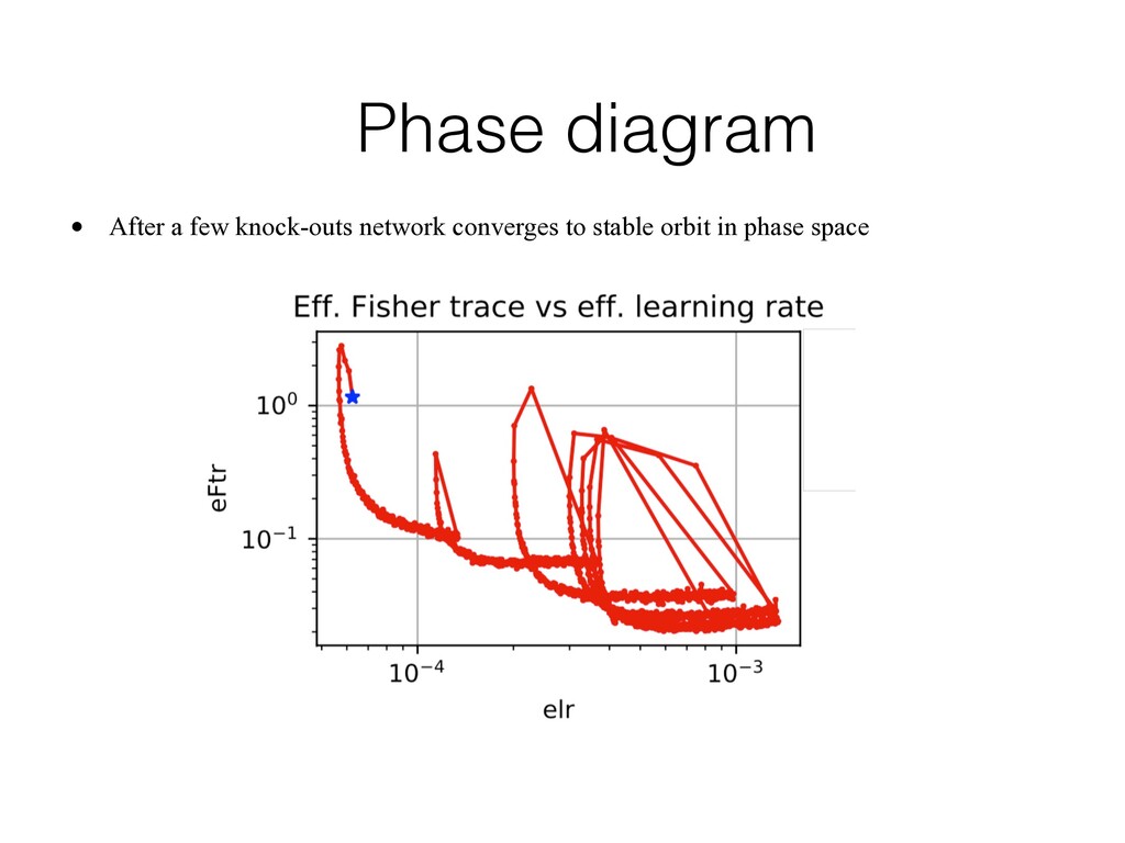
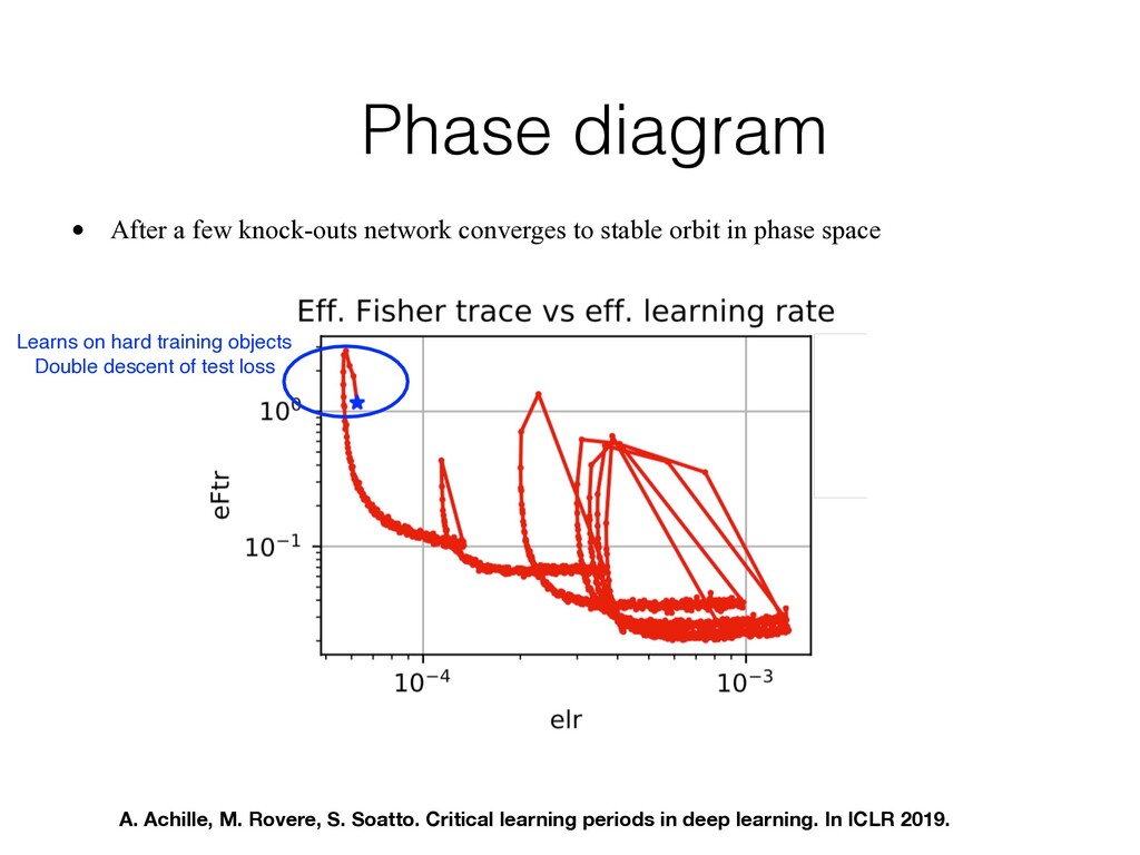
stable orbit in phase space Learns on hard training objects Double descent of test loss A. Achille, M. Rovere, S. Soatto. Critical learning periods in deep learning. In ICLR 2019.
of train loss minimum • There are multiple global minima of different curvature • For scale-invariant networks effective learning rate is important • Batch-normalization allows to automatically adapt the effective learning rate to the values which ensure good generalization
![The evolution of weight norm • The [stochastic] gradient from](https://files.speakerdeck.com/presentations/694b8f0a3ef24cf7abd2a97d8520e6cc/slide_13.jpg)