Active Subspaces: Dimension Reduction for Approximation, Integration, and Optimization

Stanford Institute for Computational and Mathematical Engineering Linear Algebra and Optimization Seminar, May 14, 2015

Transcript

1. Paul Constantine Colorado School of Mines @DrPaulynomial activesubspaces.org Qiqi Wang (MIT, AeroAstro) David Gleich (Purdue, CS) ACTIVE SUBSPACES Emerging ideas for dimension reduction in approximation, integration, and optimization DISCLAIMER: These slides are meant to complement the oral presentation. Use out of context at your own risk. This material is based upon work supported by the U.S. Department of Energy Office of Science, Office of Advanced Scientific Computing Research, Applied Mathematics program under Award Number DE-SC-0011077.
2. bookstore.siam.org/sl02/ $27 Coupon code: BKSL15
3. [ Show them that cool animation! ]
4. f( x )
5. APPROXIMATION OPTIMIZATION INTEGRATION ˜ f( x ) ⇡ f( x ) Z f( x ) ⇢ d x minimize x f( x )
6. Dimension 10 points / dimension 1 second / evaluation 1 10 10 s 2 100 ~ 1.6 min 3 1,000 ~ 16 min 4 10,000 ~ 2.7 hours 5 100,000 ~ 1.1 days 6 1,000,000 ~ 1.6 weeks … … … 20 1e20 3 trillion years (240x age of the universe) “Dimension reduction” “Better designs” “Reduced order models”
7. Key contributions of active subspaces 1.  Generalize coordinate-based reduction to linear combinations. 2.  Formalize how to properly ignore unimportant linear combinations.
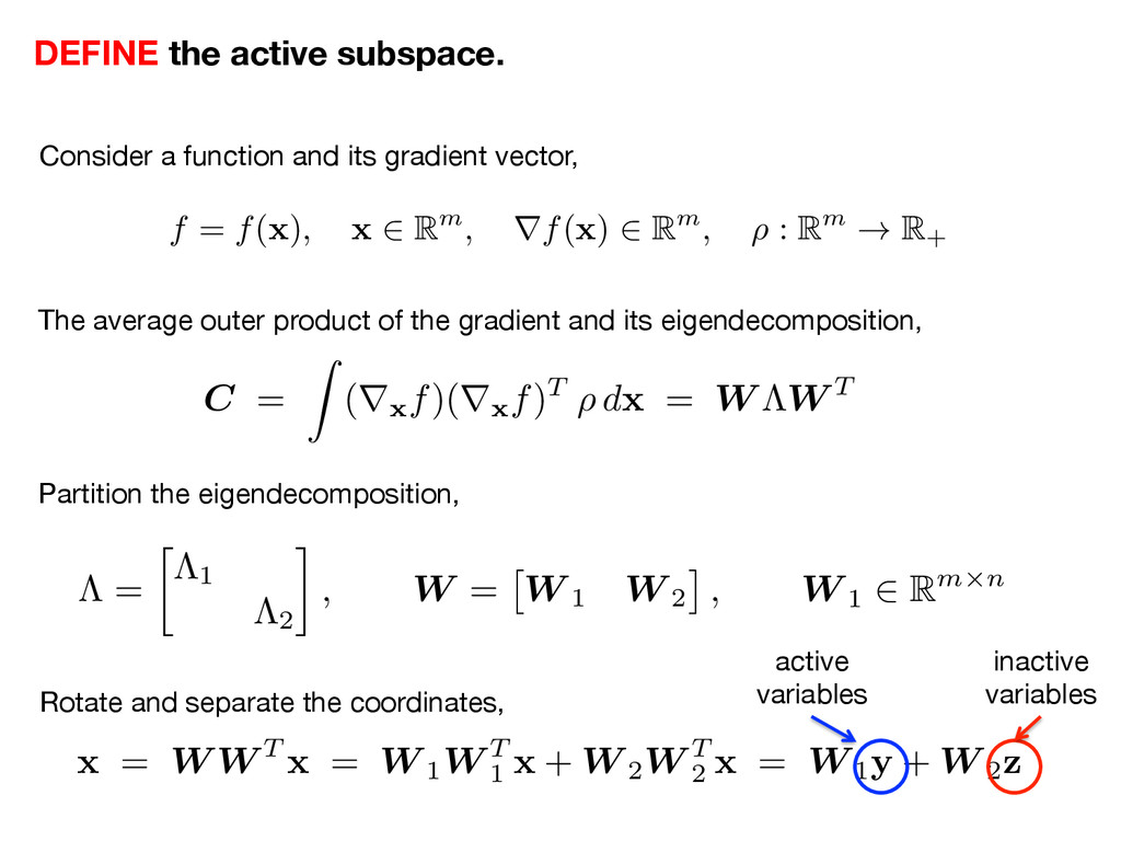
8. DEFINE the active subspace. Consider a function and its gradient vector, The average outer product of the gradient and its eigendecomposition, Partition the eigendecomposition, Rotate and separate the coordinates, ⇤ =  ⇤1 ⇤2 , W = ⇥ W 1 W 2 ⇤ , W 1 2 Rm⇥n x = W W T x = W 1W T 1 x + W 2W T 2 x = W 1y + W 2z active variables inactive variables C = Z (r x f)(r x f)T ⇢ d x = W ⇤W T f = f( x ), x 2 Rm, rf( x ) 2 Rm, ⇢ : Rm ! R +
9. Z x x T ⇢ d x Z r x f r x fT ⇢ d x VS.
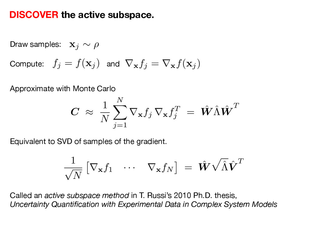
10. DISCOVER the active subspace. Draw samples: Compute: and fj = f( xj) r x fj = r x f( xj) Approximate with Monte Carlo Equivalent to SVD of samples of the gradient. Called an active subspace method in T. Russi’s 2010 Ph.D. thesis, Uncertainty Quantification with Experimental Data in Complex System Models xj ⇠ ⇢ C ⇡ 1 N N X j=1 r x fj r x fT j = ˆ W ˆ ⇤ ˆ W T 1 p N ⇥ r x f1 · · · r x fN ⇤ = ˆ W p ˆ ⇤ ˆ V T
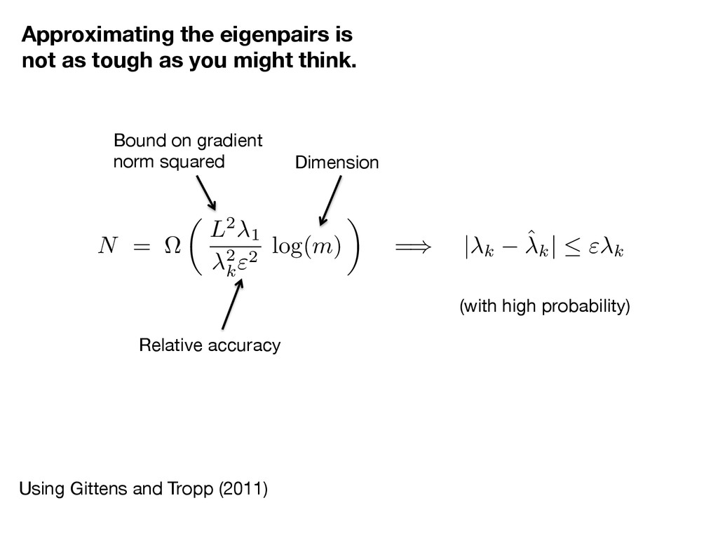
11. Using Gittens and Tropp (2011) Approximating the eigenpairs is not as tough as you might think. Bound on gradient norm squared Relative accuracy Dimension (with high probability) N = ⌦ ✓ L2 1 2 k "2 log( m ) ◆ = ) | k ˆk |  " k
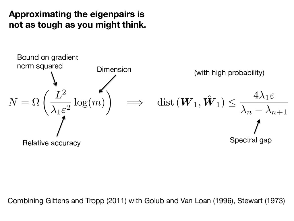
12. Approximating the eigenpairs is not as tough as you might think. Combining Gittens and Tropp (2011) with Golub and Van Loan (1996), Stewart (1973) Bound on gradient norm squared Relative accuracy Dimension (with high probability) Spectral gap N = ⌦ ✓ L2 1"2 log( m ) ◆ = ) dist ( W 1, ˆ W 1)  4 1" n n+1
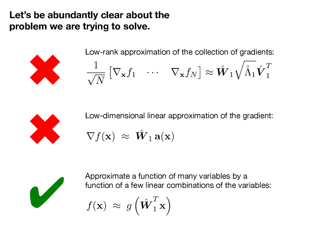
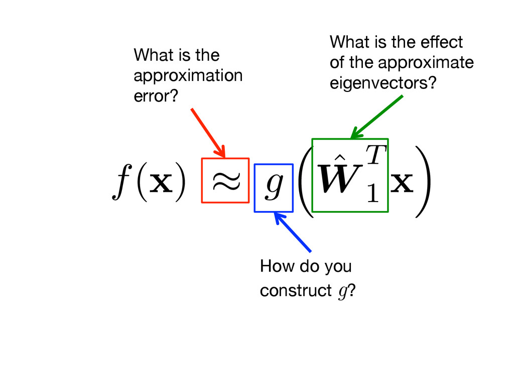
13. 1 p N ⇥ r x f1 · · · r x fN ⇤ ⇡ ˆ W 1 q ˆ ⇤1 ˆ V T 1 Low-rank approximation of the collection of gradients: Let’s be abundantly clear about the problem we are trying to solve. Low-dimensional linear approximation of the gradient: rf( x ) ⇡ ˆ W 1 a ( x ) f( x ) ⇡ g ⇣ ˆ W T 1 x ⌘ Approximate a function of many variables by a function of a few linear combinations of the variables: ✔   ✖   ✖  
14. ˜ f( x ) ⇡ f( x ) APPROXIMATION
15. f( x ) ⇡ g ⇣ ˆ W T 1 x ⌘ How do you construct g? What is the approximation error? What is the effect of the approximate eigenvectors?
16. x 2 [ 1 , 1] m, ⇢ (x) = ⇢ 2 m, x 2 [ 1 , 1] m, 0 , otherwise . Consider the following case.
17. −2 −1 0 1 2 −2 −1 0 1 2 Active Variable 1 Active Variable 2 n y = W T 1 x , 1  x  1o m = 3 The domain is a zonotope.
18. m = 5 n y = W T 1 x , 1  x  1o The domain is a zonotope.
19. m = 10 n y = W T 1 x , 1  x  1o The domain is a zonotope.
20. m = 20 n y = W T 1 x , 1  x  1o The domain is a zonotope.
21. m = 100 n y = W T 1 x , 1  x  1o The domain is a zonotope.
22. The inverse map needs regularization. y = W T 1 x , 1  x  1 forward inverse
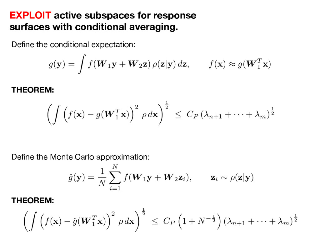
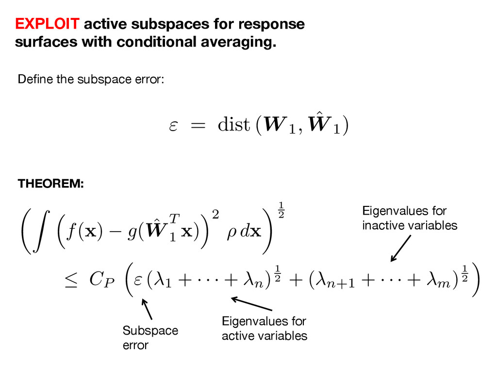
23. Define the conditional expectation: THEOREM: Define the Monte Carlo approximation: THEOREM: g( y ) = Z f(W 1y + W 2z ) ⇢( z | y ) d z , f( x ) ⇡ g(W T 1 x ) ˆ g(y) = 1 N N X i=1 f(W 1y + W 2zi), zi ⇠ ⇢(z|y) EXPLOIT active subspaces for response surfaces with conditional averaging. ✓Z ⇣ f( x ) g(W T 1 x ) ⌘2 ⇢ d x ◆1 2  CP ( n+1 + · · · + m)1 2 ✓Z ⇣ f( x ) ˆ g(W T 1 x ) ⌘2 ⇢ d x ◆1 2  CP ⇣ 1 + N 1 2 ⌘ ( n+1 + · · · + m)1 2
24. ✓Z ⇣ f( x ) g( ˆ W T 1 x ) ⌘2 ⇢ d x ◆1 2  CP ⇣ " ( 1 + · · · + n)1 2 + ( n+1 + · · · + m)1 2 ⌘ EXPLOIT active subspaces for response surfaces with conditional averaging. Subspace error Eigenvalues for active variables Eigenvalues for inactive variables Define the subspace error: " = dist (W 1, ˆ W 1) THEOREM:
25. THE BIG IDEA 1.  Choose points in the domain of g. 2.  Estimate conditional averages at each point. 3.  Construct the approximation in n < m dimensions.
26. INTEGRATION Z f( x ) ⇢ d x
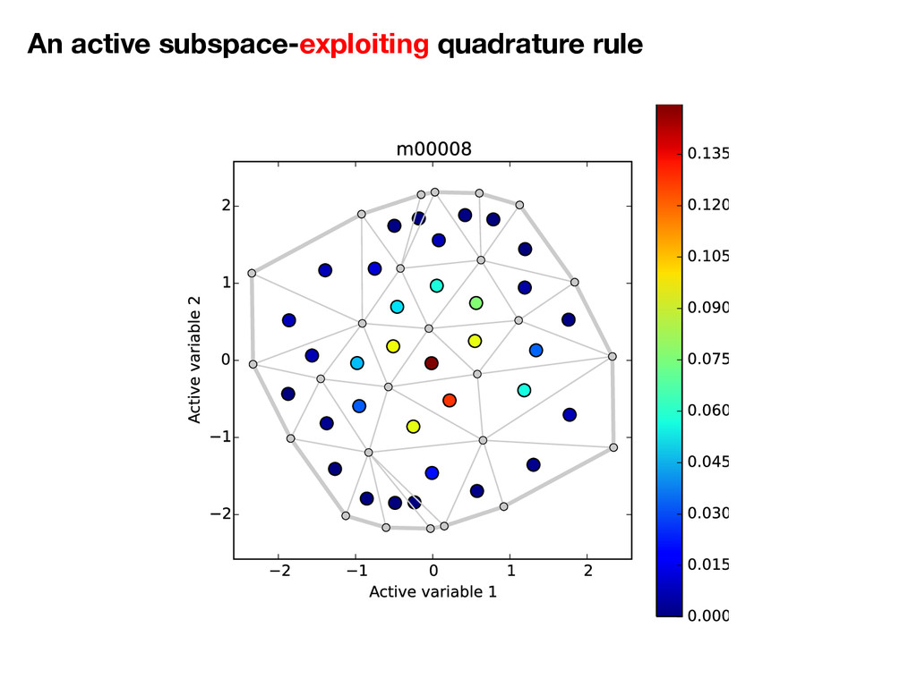
27. Z f( x ) ⇢ d x = Z Z f(W 1y + W 2z ) ⇢( z | y ) d z | {z } = g(y) ⇢( y ) d y = Z g( y ) ⇢( y ) d y ⇡ N X i=1 g( yi) wi ⇡ N X i=1 ˆ g( yi) wi Integrate in active variables. Quadrature rule in active variables. Monte Carlo in inactive variables.
28. An active subspace-exploiting quadrature rule
29. OPTIMIZATION HEURISTICS minimize x f( x )
30. y⇤ = ( argmin y g ( y ) subject to y 2 Y Assume the following structure, f( x ) = g(W T 1 x ) STRATEGY: minimize x 0 T x subject to y ⇤ = W T 1 x 1  x  1
31. −1 −0.5 0 0.5 1 −1 0 1 0 0.1 0.2 0.3 0.4 0.5 0.6 0.7 0.8 0.9 1 x1 x2 f
32. Use the active subspace to help find starting values for a gradient-based method.
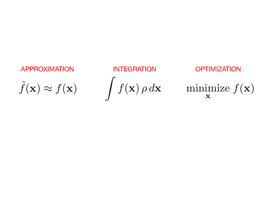
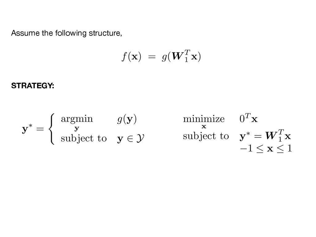
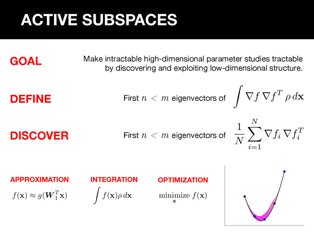
33. DEFINE ACTIVE SUBSPACES DISCOVER First n < m eigenvectors of Z rf rfT ⇢ d x 1 N N X i=1 rfi rfT i GOAL Make intractable high-dimensional parameter studies tractable by discovering and exploiting low-dimensional structure. First n < m eigenvectors of f( x ) ⇡ g(W T 1 x ) Z f( x )⇢ d x minimize x f( x ) APPROXIMATION INTEGRATION OPTIMIZATION
34. APPLICATIONS A.  ONERA M6 shape optimization (60 -> 1) B.  HyShot II scramjet uncertainty quantification (7 -> 1) C.  Photovoltaics circuit model (5 -> 1) D.  Parameterized Poisson equation (100 -> 1)
35. Active subspaces give insight into high-dimension shape design. •  ONERA M6 transonic wing (SU2) •  60 shape parameters •  (Noisy) adjoint-based gradients •  Lift and drag DIMENSION REDUCTION: 60 to 1 −2 −1 0 1 2 −0.1 0 0.1 0.2 0.3 0.4 0.5 0.6 0.7 0.8 0.9 Active Variable 1 Lift −2 −1 0 1 2 −0.1 0 0.1 0.2 0.3 0.4 0.5 0.6 0.7 0.8 0.9 Active Variable 1 Lift −2 −1 0 1 2 −0.1 0 0.1 0.2 0.3 0.4 0.5 0.6 0.7 0.8 0.9 Active Variable 1 Lift
36. Active subspaces give insight into high-dimension shape design. •  ONERA M6 transonic wing (SU2) •  60 shape parameters •  (Noisy) adjoint-based gradients •  Lift and drag DIMENSION REDUCTION: 60 to 1 −2 −1 0 1 2 0.01 0.02 0.03 0.04 0.05 0.06 0.07 0.08 0.09 Active Variable 1 Drag −2 −1 0 1 2 0.01 0.02 0.03 0.04 0.05 0.06 0.07 0.08 0.09 Active Variable 1 Drag −2 −1 0 1 2 0.01 0.02 0.03 0.04 0.05 0.06 0.07 0.08 0.09 Active Variable 1 Drag
37. Active subspaces helped us optimize an expensive scramjet model. •  Multiphysics model of hypersonic scramjet •  7 input parameters •  No gradients •  Noisy function evaluations •  2 hours per evaluation −0.5 0 0.5 1 2.35 2.4 2.45 2.5 2.55 2.6 2.65 Exit Pressure [bar] Reduced coordinate Active Variable DIMENSION REDUCTION: 7 to 1
38. Active subspaces help study a photovoltaic circuit model. DIMENSION REDUCTION: 5 to 1 Index 1 2 3 4 5 Eigenvalues 10-7 10-6 10-5 10-4 10-3 10-2 Est BI Subspace Dimension 1 2 3 4 Distance 10-3 10-2 10-1 100 Est BI Voltage (V) 0 0.2 0.4 0.6 0.8 1 1.2 Current (A) 0 0.05 0.1 0.15 0.2 0.25 0.3 I-V curves Pmax Active Variable 1 -1.5 -1 -0.5 0 0.5 1 1.5 P max (W) 0.02 0.04 0.06 0.08 0.1 0.12 0.14 0.16 •  Lumped parameter model of a single-diode solar cell •  5 parameters characterizing max power •  Finite difference gradients
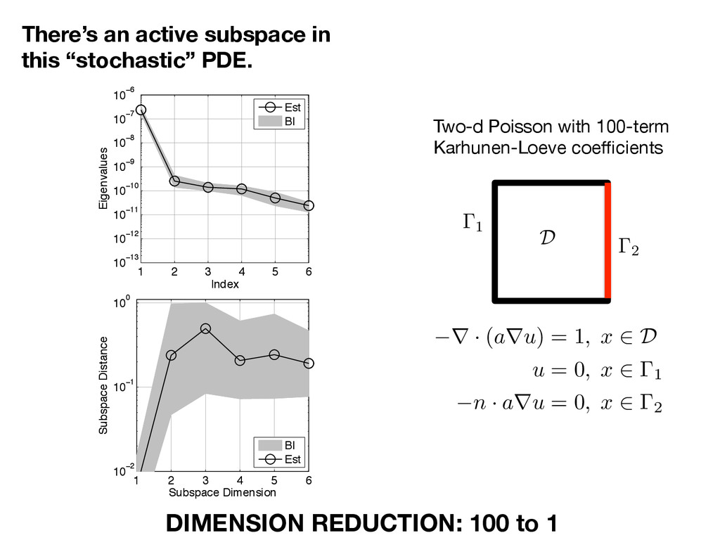
39. There’s an active subspace in this “stochastic” PDE. Two-d Poisson with 100-term Karhunen-Loeve coefficients 1 2 D r · ( a r u ) = 1 , x 2 D u = 0 , x 2 1 n · a r u = 0 , x 2 2 DIMENSION REDUCTION: 100 to 1 1 2 3 4 5 6 10−13 10−12 10−11 10−10 10−9 10−8 10−7 10−6 Index Eigenvalues Est BI 1 2 3 4 5 6 10−13 10−12 10−11 10−10 10−9 10−8 10−7 10−6 Index Eigenvalues 1 2 3 4 5 6 10−2 10−1 100 Subspace Dimension Subspace Distance BI Est 1 2 3 4 5 6 10−2 10−1 100 Subspace Dimension Subspace Distance
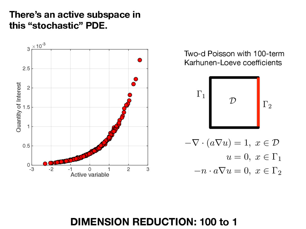
40. Two-d Poisson with 100-term Karhunen-Loeve coefficients 1 2 D Active variable -3 -2 -1 0 1 2 3 Quantity of Interest #10-3 0 0.5 1 1.5 2 2.5 3 r · ( a r u ) = 1 , x 2 D u = 0 , x 2 1 n · a r u = 0 , x 2 2 There’s an active subspace in this “stochastic” PDE. DIMENSION REDUCTION: 100 to 1
41. Python Active-subspaces Utility Library github.com/paulcon/active_subspaces
42. Questions? •  How does this relate to PCA? •  How many gradient samples do I need? •  What if I don’t have gradients? •  What kinds of models does this work on? •  What about multiple quantities of interest? •  How new is all this? Paul Constantine Colorado School of Mines activesubspaces.org @DrPaulynomial