Folding Unfolded - Polyglot FP for Fun and Profit - Haskell and Scala - Part 1

(download for perfect quality) - See how recursive functions and structural induction relate to recursive datatypes.

Follow along as the fold abstraction is introduced and explained.

Watch as folding is used to simplify the definition of recursive functions over recursive datatypes.

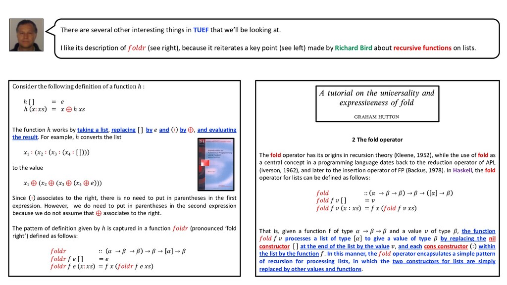
Part 1 - through the work of Richard Bird and Graham Hutton.

keywords: fold, folding, foldl, foldleft, foldr, foldright, functional programming, graham hutton, haskell, induction, left fold, recursion, recursive datatype, recursive function, richard bird, right fold, scala, structural induction

Transcript

1. See how recursive functions and structural induction relate to recursive datatypes Follow along as the fold abstraction is introduced and explained Watch as folding is used to simplify the definition of recursive functions over recursive datatypes Part 1 - through the work of Folding Unfolded Polyglot FP for Fun and Profit Haskell and Scala Graham Hutton @haskellhutt @philip_schwarz slides by https://www.slideshare.net/pjschwarz Richard Bird http://www.cs.ox.ac.uk/people/richard.bird/
2. Richard Bird @philip_schwarz This slide deck is almost entirely centered on material from Richard Bird’s fantastic book, Introduction to Functional Programming using Haskell. I hope he’ll forgive me for relying so heavily on his work, but I couldn’t resist using extensive excerpts from his compelling book to introduce and explain the concept of folding. http://www.cs.ox.ac.uk/people/richard.bird/ https://en.wikipedia.org/wiki/Richard_Bird_(computer_scientist)
3. 3.1 Natural Numbers The natural numbers are the numbers 0, 1, 2 and so on, used for counting. The type is introduced by the declaration = | is our first example of a recursive datatype declaration. The definition says that Zero is a value of , and that Succ is a value of whenever is. In particular, the constructor (short for ‘successor’), has type → . For example, each of , , ( ) is an element of . As an element of the number 7 would be represented by ( ( ( ( ( ( )))))) Every natural number is represented by a unique value of . On the other hand, not every value of represents a well- defined natural number. In fact also contains the values ⊥, ⊥, ( ⊥), and so on. These additional values will be discussed later. Let us see how to program the basic arithmetic and comparison operations on . Addition can be defined by + ∷ → → + = + = + This is a recursive definition, defining + by pattern matching on the second argument. Since every element of , apart for ⊥, is either or of the form Succ , where is an element of , the two patterns in the equations for + are disjoint and cover all numbers apart from ⊥. … Richard Bird
4. Here is how + ( ) would be evaluated: + ( ) = { second equation for +, i.e. + = + } + = { second equation for +, i.e. + = + } ( + ) = { first equation for +, i.e. + = } ( ) …it is not a practical proposition to introduce natural numbers through the datatype : arithmetic would be just too inefficient. In particular, calculating + n would require ( + 1) evaluation steps. On the other hand, counting on your fingers is a good way to understand addition. Given +, we can define ×: (×) ∷ → → × = × = × + Given ×, we can define exponentiation (↑) by (↑) ∷ → → ↑ = ↑ = ↑ × … Richard Bird
5. On the next slide we show the definitions of +, ×, and ↑ again, and have a go at implementing the three operations in Scala, together with some tests.
6. val `(+)`: Nat => Nat => Nat = m => { case Zero => m case Succ(n) => Succ(m + n) } implicit class NatOps(m: Nat){ def +(n: Nat) = `(+)`(m)(n) def ×(n: Nat) = `(×)`(m)(n) def ↑(n: Nat) = `(↑)`(m)(n) } sealed trait Nat case class Succ(n: Nat) extends Nat case object Zero extends Nat + ∷ → → + = + = + val `(×)`: Nat => Nat => Nat = m => { case Zero => Zero case Succ(n) => (m × n) + m } val `(↑)`: Nat => Nat => Nat = m => { case Zero => Succ(Zero) case Succ(n) => (m ↑ n) × m } (×) ∷ → → × = × = × + (↑) ∷ → → ↑ = ↑ = ↑ × = | ; assert(0 + 0 == 0) ; assert(Zero + Zero == Zero) ; assert(0 + 1 == 1) ; assert(Zero + Succ(Zero) == Succ(Zero)) ; assert(1 + 0 == 1) ; assert(Succ(Zero) + Zero == Succ(Zero)) ; assert(1 + 1 == 2) ; assert(Succ(Zero) + Succ(Zero) == Succ(Succ(Zero))) ; assert(2 + 3 == 5) ; assert(Succ(Succ(Zero)) + Succ(Succ(Succ(Zero))) == Succ(Succ(Succ(Succ(Succ(Zero)))))) ; assert(0 * 0 == 0) ; assert((Zero × Zero) == Zero) ; assert(1 * 0 == 0) ; assert((Succ(Zero) × Zero) == Zero) ; assert(0 * 1 == 0) ; assert((Zero × Succ(Zero)) == Zero) ; assert(1 * 1 == 1) ; assert((Succ(Zero) × Succ(Zero)) == Succ(Zero)) ; assert(1 * 2 == 2) ; assert((Succ(Zero) × Succ(Succ(Zero))) == Succ(Succ(Zero))) ; assert(2 * 3 == 6) ; assert((Succ(Succ(Zero)) × Succ(Succ(Succ(Zero)))) == Succ(Succ(Succ(Succ(Succ(Succ(Zero))))))) ; assert(Math.pow(1,0) == 1) ; assert( (Succ(Zero) ↑ Zero) == Succ(Zero) ) ; assert(Math.pow(2,2) == 4) ; assert( (Succ(Succ(Zero)) ↑ Succ(Succ(Zero))) == Succ(Succ(Succ(Succ(Zero)))) )
7. The remaining arithmetic operation common to all numbers is subtraction (−). However, subtraction is a partial operation on natural numbers. The definition is − ∷ → → − = − = − This definition uses pattern matching on both arguments; taken together, the patterns are disjoint but not exhaustive. For example, − ( ) = { second equation for −, i.e. − = − } − = { case exhaustion } ⊥ The hint ‘case exhaustion’ in the last step indicates that no equation for − has a pattern that matches ( − ). More generally, − = ⊥ if < . The partial nature of subtraction on the natural numbers is the prime motivation for introducing the integer numbers; over the integers, − is a total operation. ...Finally, here are two more examples of programming with . The factorial and Fibonacci functions are defined by ∷ → = = × ∷ → = = = + Richard Bird
8. See the next slide for a Scala implementation of the − operation.
9. − ∷ → → − = − = − val `(-)`: Nat => Nat => Nat = m => n => (m,n) match { case (_,Zero) => m case (Succ(x),Succ(y)) => x - y } ; assert(0 - 0 == 0) ; assert(Zero - Zero == Zero) ; assert(1 - 0 == 1) ; assert(Succ(Zero) - Zero == Succ(Zero)) ; assert(5 - 3 == 2) ; assert(Succ(Succ(Succ(Succ(Succ(Zero))))) - Succ(Succ(Succ(Zero))) == Succ(Succ(Zero))) ; assert(3 - 5 == -2) ; assert( Try { Succ(Succ(Succ(Zero))) - Succ(Succ(Succ(Succ(Succ(Zero))))) }.toString.startsWith( "Failure(scala.MatchError: (Zero,Succ(Succ(Zero)))" ) ) No equation for − has a pattern that matches ( − ). Similarly for ( − ( )), ( − (( ))), etc. More generally, − = ⊥ if < . − throws scala.MatchError if < .
10. @philip_schwarz On the next slide we show the definitions of , and again, and have a go at implementing the two functions in Scala, together with some tests.
11. val fact: Nat => Nat = { case Zero => Succ(Zero) case Succ(n) => Succ(n) × fact(n) } ∷ → = = × ∷ → = = = + val fib: Nat => Nat = { case Zero => Zero case Succ(Zero) => Succ(Zero) case Succ(Succ(n)) => fib(Succ(n)) + fib(n) } def factorial(n: Int): Int = if (n == 0) 1 else n * factorial(n-1) ; assert(factorial(0) == 1) ; assert(fact(Zero) == Succ(Zero)) ; assert(factorial(1) == 1) ; assert(fact(Succ(Zero)) == Succ(Zero)) ; assert(factorial(2) == 2) ; assert(fact(Succ(Succ(Zero))) == Succ(Succ(Zero))) ; assert(factorial(3) == 6) ; assert(fact(Succ(Succ(Succ(Zero)))) == Succ(Succ(Succ(Succ(Succ(Succ(Zero))))))) def fibonacci(n: Int): Int = if (n == 0 || n == 1) n else fibonacci(n-1) + fibonacci(n-2) ; assert(fibonacci(0) == 0) ; assert(fib(Zero) == Succ(Zero)) ; assert(fibonacci(1) == 1) ; assert(fib(Succ(Zero)) == Succ(Zero)) ; assert(fibonacci(2) == 1) ; assert(fib(Succ(Succ(Zero))) == Succ(Zero)) ; assert(fibonacci(3) == 2) ; assert(fib(Succ(Succ(Succ(Zero)))) == Succ(Succ(Zero))) ; assert(fibonacci(4) == 3) ; assert(fib(Succ(Succ(Succ(Succ(Zero))))) == Succ(Succ(Succ(Zero)))) ; assert(fibonacci(5) == 5) ; assert(fib(Succ(Succ(Succ(Succ(Succ(Zero)))))) == Succ(Succ(Succ(Succ(Succ(Zero)))))) ; assert(fibonacci(6) == 8) ; assert(fib(Succ(Succ(Succ(Succ(Succ(Zero)))))) == Succ(Succ(Succ(Succ(Succ(Succ(Succ(Succ(Zero)))))))))
12. 3.1.1 Partial numbers Let us now return to the point about there being extra values in . The values ⊥, ⊥, ( ⊥), … are all different and each is also a member of . That they exist is a consequence of three facts: i. ⊥ is an element of because every datatype declaration introduces at least one extra value, the undefined value of the type. ii. constructor functions of a datatype are assumed to be nonstrict iii. is an element of Nat, whenever is To appreciate why these extra values are different from one another, suppose we define ∷ by the equation = . Then ? < {Interrupted!} ? < ? < {Interrupted!} ? < ( ) One can interpret the extra values in the following way: ⊥ corresponds to the natural number about which there is absolutely no information; ⊥ to the natural number about which the only information is that it is greater than ; ( ⊥) to the natural number about which the only information is that it is greater than ; and so on. Richard Bird
13. There is also one further value of , namely the ‘infinite’ number: ( ( ( … ))) This number can be defined by ∷ = It is different from all the other numbers, because it is the only number for which < returns for all finite numbers . In this sense, is the largest element of . If we request the value of , then we obtain ? ( ( ( ( {!} The number satisfies other properties, in particular + = , for all numbers . The dual equation + = holds only for finite numbers . We will see how to prove assertions such as these in the next section. To summarise this discussion, we can divide the values of into three classes: • The finite numbers, those that correspond to well-defined natural numbers. • The partial numbers, ⊥, ⊥, and so on. • The infinite numbers, of which there is just one, namely . We will see that this classification holds true of all recursive types. There will be the finite elements of the type, the partial elements, and the infinite elements. Although the infinite natural number is not of much use, the same is not true of the infinite values of other datatypes. … Richard Bird
14. Note that when in this slide deck we mention the concepts of ⊥ and , it is mainly in a Haskell context, as we did in the last two slides. In particular, we won’t be modelling ⊥ and in any of the Scala code you’ll see throughout the deck.
15. 3.2 Induction In order to reason about the properties of recursively defined functions over a recursive datatype, we can appeal to a principle of structural induction. In the case of , the principle of structural induction can be defined as follows: In order to show that some property () holds for each finite number of , it is sufficient to show: Case (). That () holds. Case ( ). That if () holds, then ( ) holds also. Induction is valid for the same reason that recursive definitions are valid: every finite number is either or of the form , where is a finite number. If we prove the first case, then we have shown that the property is true for ; If we also prove the second case, then we have shown that the property is true for , since it is true for . But now, by the same argument, it is true for , and so on. The principle needs to be extended if we want to assert that some proposition is true for all elements of , but we postpone discussion of this point for the following section. As an example, let’s prove that + = for all finite numbers . Recall that + is defined by + = + = + The first equation asserts that is a right unit of +. In general, is a left unit of ⊕ if ⊕ = for all , and a right unit of if ⊕ = for all . If is both a left unit and a right unit of an operator ⊕, then it is called the unit of ⊕. The terminology is appropriate since only one value can be both a left and right unit. So, by proving that is a left unit , we have proved that is the unit of +. Richard Bird
16. Proof. The proof is by induction on . More precisely, we take for () the assertion that + = . This equation is referred to as the induction hypothesis. Case (). We have to show + = , which is immediate from the first equation defining +. Case ( ). We have to show that + = , which we do by simplifying the left-hand expression: + = { second equation for +, i.e. + = + } ( + ) = { induction hypothesis} ☐ This example shows the format we will use for inductive proofs, laying out each case separately and using a ☐ to mark the end. The very last step made use of the induction hypothesis, which is allowed by the way induction works. … 3.2.1 Full Induction In the form given above, the induction principle for suffices only to prove properties of the finite members of . If we want to show that a property also hold for every partial number, then we have to prove three things: Case (⊥). That (⊥) holds. Case (). That () holds. Case ( ). That if () holds, then ( ) holds also. We can omit the second case, but then we can conclude only that () holds for every partial number. The reason the principle is valid is that is that every partial number is either ⊥ or of the form for some partial number . Richard Bird
17. To illustrate, let us prove the somewhat counterintuitive result that + = for all numbers and all partial numbers . Proof. The proof is by partial number induction on . Case (⊥). The equation + ⊥ = ⊥ follows at once by case exhaustion in the definition of +. That is, ⊥ does not match either of the patterns or . Case ( ). For the left-hand side, we reason + = { second equation for +, i.e. + = + } ( + ) = { induction hypothesis} Since the right-hand side is also , we are done. 3.2.2 Program synthesis In the proofs above we defined some functions and then used induction to prove a certain property. We can also view induction as a way to synthesise definitions of functions so that they satisfy the properties we want. Let us illustrate with a simple example. Suppose we specify subtraction of natural numbers by the condition + − = for all and . The specification does not give a constructive definition of − , merely a property that it has to satisfy. However, we can do an induction proof on of the equation above, but view the calculation as a way of generating a suitable definition of − . Richard Bird
18. Unlike previous proofs, we reason with the equation as a whole, since simplification of both sides independently is not possible if we do not know what all the rules of simplification are. Case (). We reason + − = ≡ { first equation for +, i.e. + = } − = Hence we can take − = to satisfy the case. The symbol ≡ is used to separate steps of the calculation since we are calculating with mathematical assertions, not with values of a datatype. Case ( ). We reason + − = ≡ { second equation for +, i.e. + = + } + − = ≡ { hypothesis + − = } + − = + − Replacing + in the last equation by , we can take − = − to satisfy the case. Hence we have derived − = − = − This is the program for − seen earlier. Richard Bird
19. After that look at structural induction, it is finally time to see how Richard Bird introduces the concept of folding.
20. 3.3 The fold function Many of the recursive definitions seen so far have a common pattern, exemplified by the following definition of a function : ∷ → = = ℎ Here, is some type, is an element of , and ℎ ∷ → . Observe that works by taking an element of and replacing by and by ℎ. For example, takes ( ( )) to ℎ (ℎ (ℎ )) The two equations for can be captured in terms of a single function, , called the function for . The definition is ∷ → → → → ℎ = ℎ = ℎ ℎ In particular, we have + = × = + ↑ = × It follows also that the identity function on satisfies = . A suitable function can be defined for every recursive type, and we will see other functions in the following chapters. Richard Bird
21. + ∷ → → + = + = + (×) ∷ → → × = × = × + (↑) ∷ → → ↑ = ↑ = ↑ × + ∷ → → + = (×) ∷ → → × = + (↑) ∷ → → ↑ = × ∷ → → → → ℎ = ℎ = ℎ ℎ @philip_schwarz Just to reinforce the ideas on the previous slide, here are the original definitions of +, × and ↑, and next to them, the new definitions in terms of . And the next slide is the same but in terms of Scala code.
22. val `(+)`: Nat => Nat => Nat = m => { case Zero => m case Succ(n) => Succ(m + n) } val `(×)`: Nat => Nat => Nat = m => { case Zero => Zero case Succ(n) => (m × n) + m } val `(↑)`: Nat => Nat => Nat = m => { case Zero => Succ(Zero) case Succ(n) => (m ↑ n) × m } val `(×)`: Nat => Nat => Nat = m => n => foldn((x:Nat) => x + m, Zero, n) def foldn[A](h: A => A, c: A, n: Nat): A = n match { case Zero => c case Succ(n) => h(foldn(h,c,n)) } val `(↑)`: Nat => Nat => Nat = m => n => foldn((x:Nat) => x × m, Succ(Zero), n) val `(+)`: Nat => Nat => Nat = m => n => foldn(Succ,m,n)
23. In the examples above, each instance of also returned an element of . In the following two examples, returns an element of (, ): ∷ → = Š (, ) where , = ( , () × ) ∷ → = Š (, ) where , = (, + ) The function computes the factorial function and function computes the Fibonacci function. Each program works by first computing a more general result, namely an element of (, ), and then extracts the required result. In fact, , = , , = , These equations can be proved by induction. The program for is more efficient than a direct recursive definition. The recursive program requires an exponential number of + operations, while the program above requires only a linear number. We will discuss efficiency in more detail in chapter 7, where the programming technique that led to the invention of the new program for will be studied in a more general setting. There are two advantages of writing recursive definitions in terms of . Firstly, the definition is shorter; rather than having to write down two equations, we have only to write down one. Secondly, it is possible to prove general properties of and use them to prove properties of specific instantiations. In other words, rather than having to write down many induction proofs, we have only to write down one. Richard Bird
24. @philip_schwarz The next slide shows the original definitions of the factorial and Fibonacci functions, and next to them, the new definitions in terms of . And the slide after that is the same but in terms of Scala code.
25. ∷ → = = × ∷ → = 7 (, ) where , = (, + ) ∷ → = 7 (, ) where , = ( , () × ) ∷ → = = = + ∷ → → → → ℎ = ℎ = ℎ ℎ
26. def fact(n: Nat): Nat = { def snd(pair: (Nat, Nat)): Nat = pair match { case (_,n) => n } def f(pair: (Nat, Nat)): (Nat, Nat) = pair match { case (m,n) => (Succ(m), Succ(m) × n) } snd( foldn(f, (Zero, Succ(Zero)), n) ) } def fib(n: Nat): Nat = { def fst(pair: (Nat, Nat)): Nat = pair match { case (n,_) => n } def g(pair: (Nat, Nat)): (Nat, Nat) = pair match { case (m,n) => (n, m + n) } fst( foldn(g, (Zero, Succ(Zero)), n) ) } val fact: Nat => Nat = { case Zero => Succ(Zero) case Succ(n) => Succ(n) × fact(n) } val fib: Nat => Nat = { case Zero => Zero case Succ(Zero) => Succ(Zero) case Succ(Succ(n)) => fib(Succ(n)) + fib(n) } def foldn[A](h: A => A, c: A, n: Nat): A = n match { case Zero => c case Succ(n) => h(foldn(h,c,n)) }
27. Now let’s have a very quick look at the datatype for lists, and at induction over lists.
28. 4.1.1 Lists as a datatype A list can be constructed from scratch by starting with the empty list and successively adding elements one by one. One can add elements to the front of the list, or to the rear, or to somewhere in the middle. In the following datatype declaration, nonempty lists are constructed by adding elements to the front of the list: = | ( ) …The constructor (short for ‘construct’ – the name goes back to the programming language LISP) adds an element to the front of the list. For example, the list 1,2,3 would be represented as the following element of : 1 ( 2 ( 3 )) In functional programming, lists are defined as elements of . The syntax [] is used instead of , the constructor is written as [ ], and the constructor is written as infix operator (∶). Moreover, (∶) associates to the right, so 1,2,3 = 1: 2: 3: [ ] = 1 ∶ 2 ∶ 3 ∶ [ ] In other words, the special syntax on the left can be regarded as an abbreviation for the syntax on the right, which is also special, but only by virtue of the fact that the constructors are given nonstandard names. Like functions over other datatypes, functions over lists can be defined by pattern matching. Richard Bird
29. Before moving on to the topic of induction over lists, Richard Bird gives an example of a function defined over lists using pattern matching, but the function he chooses is the equality function, whereas we are going to choose the sum function, just to keep things simpler. ∷ [] → [ ] = 0 : = + ( ) val sum : List[Int] => Int = { case Nil => 0 case x :: xs => x + sum(xs) } assert( sum( 1 :: (2 :: (3 :: Nil)) ) == 6)
30. sealed trait Nat case class Succ(n: Nat) extends Nat case object Zero extends Nat sealed trait List[+A] case class Cons[+A](head: A, tail: List[A]) extends List[A] case object Nil extends List[Nothing] val `(+)`: Nat => Nat => Nat = m => { case Zero => m case Succ(n) => Succ(m + n) } implicit class NatSyntax(m: Nat){ def +(n: Nat) = `(+)`(m)(n) } val sum: List[Nat] => Nat = { case Nil => Zero case Cons(x, xs) => x + sum(xs) } assert( sum( Cons( Succ(Zero), // 1 Cons( Succ(Succ(Zero)), // 2 Cons( Succ(Succ(Succ(Zero))), // 3 Nil))) ) == Succ(Succ(Succ(Succ(Succ(Succ(Zero))))))) // 6 ∷ → = = + ( ) + ∷ → → + = + = + = | α = | α ( α) Same as on the previous slide, but this time using Nat rather than Int, just for fun.
31. 4.1.2 Induction over Lists Recall from section 3.2 that, for the datatype of natural numbers, structural induction is based on three cases: every element of is either ⊥, or , or else has the form for some element of . Similarly, structural induction on lists is also based on on three cases: every list is either the undefined list ⊥, the empty list [ ], or else has the form : for some and list . To show by induction that a proposition () holds for all lists it suffices therefore to establish three cases: Case (⊥). That (⊥) holds. Case ([ ]). That ([ ]) holds. Case : . That if () holds, then (: ) also holds for every . If we prove only the second two cases, then we can conclude only that () holds for every finite list; if we prove only the first and third cases. Then we can conclude only that () holds for every partial list. If takes the form of an equation, as all of our laws do, then proving the first and third cases is sufficient to show that () holds for every infinite list. Partial lists and infinite lists are described in the following section. Examples of induction proofs are given throughout the remainder of the chapter. Richard Bird
32. Richard Bird provides other examples of recursive functions over lists. Let’s see some of them: list concatenation, flattening of lists of lists, list reversal and length of a list. When looking at the first one, i.e. concatenation, let’s also see an example of proof by structural induction on lists. @philip_schwarz
33. 4.2.1 Concatenation Two lists can be concatenated to form one longer list. This function is denoted by the binary operator ⧺ (pronounced ‘concatenate’). As two simple examples, we have ? 1,2,3 ⧺ 4,5 1,2,3,4,5 ? 1,2 ⧺ ⧺ 1 1,2,1 The formal definition of ⧺ is (⧺) ∷ [α] → [α] → [α] ⧺ = : ⧺ = ∶ ( ⧺ ) Concatenation takes two lists, both of the same type, and produces a third list, again of the same type. Hence the type assignment. The definition of ⧺ is by pattern matching on the left-hand argument; the two patterns are disjoint and cover all cases, apart from the undefined list ⊥. It follows by case exhaustion that ⊥ ⧺ = ⊥. However, it is not the case that ⧺ ⊥ = ⊥. For example, ? 1,2,3 ⧺ 1,2,3{!} The list 1,2,3 ⧺ ⊥ is a partial list; In full form it is the list 1: 2: 3: ⊥. The evaluator can compute the first three elements, but thereafter it goes into a nonterminating computation, so we interrupt it. The second equation for ⧺ is very succinct and requires some thought. Once one has come to grips with the definition of ⧺, one Richard Bird
34. has understood a good deal about how lists work in functional programming. Note that the number of steps required to compute ⧺ is proportional to the number of elements in . 1, 2 ⧺ 3, 4, 5 = { notation} (1 ∶ 2 ∶ ⧺ (3 ∶ (4 ∶ 5 ∶ [ ] )) = { second equation for ⧺, i.e. : ⧺ = ∶ ( ⧺ ) } 1 ∶ ( 2 ∶ ⧺ (3 ∶ (4 ∶ 5 ∶ [ ] ))) = { second equation for ⧺ } 1 ∶ (2 ∶ ( ⧺ (3 ∶ (4 ∶ 5 ∶ [ ] )))) = { first equation for ⧺ i.e. , ⧺ = } 1 ∶ (2 ∶ (3 ∶ (4 ∶ 5 ∶ [ ] ))) = { notation} 1, 2, 3, 4, 5 Concatenation is an associative operation with unit : ⧺ ⧺ = ⧺ ( ⧺ ) ⧺ = ⧺ = Let us now prove by induction that ⧺ is associative. Proof. The proof is by induction on . Case (⊥). For the left-hand side, we reason ⊥ ⧺ ( ⧺ ) = { case exhaustion} ⊥ ⧺ = { case exhaustion} ⊥ Richard Bird
35. The right-hand side simplifies to ⊥ as well, establishing the case. Case ([ ]). For the left hand side, we reason [ ] ⧺ ( ⧺ ) = { first equation for ⧺ i.e. , ⧺ = } ( ⧺ ) The right-hand side simplifies to( ⧺ ) as well, establishing the case. Case ∶ . For the left hand side, we reason ((x ∶ ) ⧺ ) ⧺ = { second equation for ⧺, i.e. : ⧺ = ∶ ( ⧺ ) } ( ∶ ⧺ ) ⧺ = { second equation for ⧺ } ∶ ( ⧺ ⧺ ) = { induction hypothesis } ∶ ( ⧺ ⧺ ) For the right-hand side we reason (x ∶ ) ⧺ ( ⧺ ) = { second equation for ⧺, i.e. ∶ ⧺ = ∶ ( ⧺ ) } ∶ ( ⧺ ( ⧺ )) The two sides are equal, establishing the case. …Note that associativity is proved for all lists, finite, partial or infinite. Hence we can assert that ⧺ is associative without qualification…. Richard Bird
36. 4.2.2 Concat Concatenation performs much the same function for lists as the union operator ∪ does for sets. A companion function is concat, which concatenates a list of lists into one long list. This function, which roughly corresponds to the big-union operator ⋃ for sets of sets, is defined by concat ∷ [ α ] → [α] concat = concat : = ⧺ For example, ?concat [ 1, 2 , , 3, 2,1 ] 1,2,3,2,1 4.2.3 Reverse Another basic function on lists is reverse, the function that reverses the order of elements in a finite list. For example: ? reverse “Madam, I’m Adam.” “.MadA m’I ,madaM” The definition is reverse ∷ α → [α] reverse = reverse ∶ = ⧺ [] In words, to reverse a list ∶ , one reverses , and then adds to the end. As a program, the above definition is not very Richard Bird
37. efficient: on a list of length , it will need a number of reduction steps proportional to 2 to deliver the reversed list. The first element will be appended to the end of a list of length − 1 , which will take about − 1 steps, the second element will be appended to a list of length − 2 , taking − 2 steps, and so on. The total time is therefore about − 1 + − 2 + ⋯ 1 = ( − 1)/2 steps A more precise analysis is given in chapter 7, and a more efficient program for reverse is given in section 4.5. 4.2.2 Length The length of a list is the number of elements it contains: ℎ ∷ [α] → ℎ [ ] = 0 ℎ : = 1 + ℎ The nature of the list element is irrelevant when computing the length of a list, whence the type assignment. For example, ? ℎ [, ] 2 However, not every list has a well-defined length. In particular, the partial lists ⊥, ∶ ⊥, ∶ ∶ ⊥, and so on, have an undefined length. Only finite lists have well-defined lengths. The list ⊥, ⊥ is a finite list, not a partial list, because it is the list ⊥ ∶ ⊥ ∶ [ ], which ends in [ ], not ⊥. The computer cannot produce the elements, but it can produce the length of the list. … Richard Bird
38. 4.3 Map and filter Two useful functions on lists are map and £ilter. The function map applies a function to each element of a list. For example ? ap square [9, 3] ? ap (<3) [1, 2, 3] ? ap nextLetter “HAL” [81, 9] [, , ] “IBM” The definition is map ∷ (α → ) → [α] → [] map f = map f ∶ = ∶ map … 4.3 filter The second function, £ilter, takes a Boolean function and a list and returns that sublist of whose elements satisfy p. For example, ? £ilter even [1,2,4,5,32] ? (sum Š map square Š £ilter even) [1. . 10] [2,4,32] 220 The last example asks for the sum of the squares of the even integers in the range 1..10. The definition of filter is £ilter ∷ (α → ) → [α] → [α] £ilter p = £ilter p ∶ = ∶ £ilter p £ilter p … Richard Bird
39. Now let’s look at fold functions over lists.
40. 4.5 The fold functions We have seen in the case of the datatype that many recursive definitions can be expressed very succinctly using a suitable operator. Exactly the same is true of lists. Consider the following definition of a function ℎ : ℎ [ ] = ℎ : = ⊕ ℎ The function ℎ works by taking a list, replacing [ ] by and ∶ by ⊕, and evaluating the result. For example, ℎ converts the list 1 ∶ (2 ∶ 3 ∶ 4 ∶ ) to the value 1 ⊕ (2 ⊕ (3 ⊕ 4 ⊕ )) Since ∶ associates to the right, there is no need to put in parentheses in the first expression. However, we do need to put in parentheses in the second expression because we do not assume that ⊕ associates to the right. The pattern of definition given by ℎ is captured in a function (prounced ‘fold right’) defined as follows: ∷ → → → → → = : = We can now write h = ⊕ . The first argument of is a binary operator that takes an -value on its left and an a – value on its right, and delivers a –value. The second argument of is a -value. The third argument is of type , and the result is of type . In many cases, and will be instantiated to the same type, for instance when ⊕ denotes an associative operation. Richard Bird
41. In the next slide we look at how some of the recursively defined functions on lists that we have recently seen can be redefined in terms of . To aid comprehension, I have added the original function definitions next to the new definitions in terms of . For reference, I also added the definition of .
42. The single function foldr can be used to define almost every function on lists that we have met so far. Here are just some examples: concat ∷ [ α ] → [α] concat = (⧺) [ ] reverse ∷ α → [α] reverse = = ⧺ [] ℎ ∷ [α] → ℎ = 0 = 1 + … ∷ [] → = + 0 map ∷ (α → ) → [α] → [] map = Š = ∶ … concat ∷ [ α ] → [α] concat = concat : = ⧺ reverse ∷ α → [α] reverse = reverse ∶ = ⧺ [] ℎ ∷ [α] → ℎ [ ] = 0 ℎ : = 1 + ℎ ∷ [] → [ ] = 0 : = + ( ) map ∷ (α → ) → [α] → [] map f = map f ∶ = ∶ map ∷ → → → → → = : = Richard Bird
43. On the next slide, the same code translated into Scala @philip_schwarz
44. def foldr[A,B](f: A => B => B)(e: B)(xs: List[A]): B = xs match { case Nil => e case x::xs => f(x)(foldr(f)(e)(xs)) } def concatenate[A]: List[A] => List[A] => List[A] = xs => ys => xs match { case Nil => ys case x :: xs => x :: concatenate(xs)(ys) } def concat[A]: List[List[A]] => List[A] = foldr(concatenate[A])(Nil) def reverse[A]: List[A] => List[A] = { def snoc[A]: A => List[A] => List[A] = x => xs => concatenate(xs)(List(x)) foldr(snoc[A])(Nil) } def length[A]: List[A] => Int = { def oneplus[A]: A => Int => Int = x => n => 1 + n foldr(oneplus)(0) } val sum: List[Int] => Int = { val plus: Int => Int => Int = a => b => a + b foldr(plus)(0) } def map[A,B]: (A => B) => List[A] => List[B] = { def cons: B => List[B] => List[B] = x => xs => x :: xs f => foldr(cons compose f)(Nil) } ∷ → → → → → = : = (⧺) ∷ [α] → [α] → [α] ⧺ = : ⧺ = ∶ ( ⧺ ) concat ∷ [ α ] → [α] concat = (⧺) [ ] reverse ∷ α → [α] reverse = = ⧺ [] ℎ ∷ [α] → ℎ = 0 = 1 + ∷ [] → = + 0 map ∷ (α → ) → [α] → [] map = T = ∶
45. assert( concatenate(List(1,2,3))(List(4,5)) == List(1,2,3,4,5) ) assert( concat(List(List(1,2), List(3), List(4,5))) == List(1,2,3,4,5) ) assert( reverse(List(1,2,3,4,5)) == List(5,4,3,2,1) ) assert( length(List(0,1,2,3,4,5)) == 6 ) assert( sum(List(2,3,4)) == 9 ) val mult: Int => Int => Int = a => b => a * b assert( map(mult(10))(List(1,2,3)) == List(10,20,30)) Here a some sample tests for the Scala functions on the previous slide.
46. It turns out that if it is possible to define a function on lists both using a recursive definition and using a definition in terms of , then there is a technique that can be used to go from the recursive definition to the definition using . I came across the technique in the following paper by the author of Programming in Haskell: The tutorial (which I shall be referring to as TUEF), shows how to apply the technique to the sum function and the map function, which is the subject of the next five slides. Note: in the paper, the function is referred to as . @philip_schwarz
47. 3 The universal property of fold As with the fold operator itself, the universal property of also has its origins in recursion theory. The first systematic use of the universal property in functional programming was by Malcolm (1990a), in his generalisation of Bird and Meerten’s theory of lists (Bird, 1989; Meertens, 1983) to arbitrary regular datatypes. For finite lists, the universal property of can be stated as the following equivalence between two definitions for a function that processes lists: = ⟺ = ∶ = In the right-to-left direction, substituting = into the two equations for gives the recursive definition for . Conversely, in the left-to-right direction the two equations for g are precisely the assumptions required to show that = using a simple proof by induction on finite lists (Bird, 1998). Taken as a whole, the universal property states that for finite lists the function is not just a solution to its defining equations, but in fact the unique solution…. The universal property of can be generalised to handle partial and infinite lists (Bird, 1998), but for simplicity we only consider finite lists in this article. Graham Hutton @haskellhutt
48. 3.3 Universality as a definition principle As well as being used as a proof principle, the universal property of can also be used as a definition principle that guides the transformation of recursive functions into definitions using . As a simple first example, consider the recursively defined function that calculates the sum of a list of numbers: ∷ → = 0 ∶ = + Suppose now that we want to redefine using . That is, we want to solve the equation = for a function f and a value . We begin by observing that the equation matches the right-hand side of the universal property, from which we conclude that the equation is equivalent to the following two equations: = ∶ = ( ) From the first equation and the definition of , it is immediate that = 0. = ⟺ = ∶ = Graham Hutton @haskellhutt universal property of
49. From the second equation, we calculate a definition for as follows: ∶ = ( ) ⇔ { Definition of } + = ( ) ⇐ { † Generalising ( ) to } + = ⇔ { Functions } = (+) That is, using the universal property we have calculated that: = + 0 Note that the key step (†) above in calculating a definition for is the generalisation of the expression to a fresh variable . In fact, such a generalisation step is not specific to the function, but will be a key step in the transformation of any recursive function into a definition using in this manner. ∷ → = 0 ∶ = + = ∶ = ( ) Graham Hutton @haskellhutt
50. Of course, the example above is rather artificial, because the definition of using is immediate. However, there are many examples of functions whose definition using is not so immediate. For example, consider the recursively defined function that applies a function to each element of a list: ∷ → → → = ∶ = ∶ To redefine using we must solve the equation = for a function and a value . By appealing to the universal property, we conclude that this equation is equivalent to the following two equations: = ∶ = ( ) From the first equation and the definition of it is immediate that = [ ]. Graham Hutton @haskellhutt = ⟺ = ∶ = substitute for and for universal property of
51. From the second equation, we calculate a definition for as follows: ∶ = ( ) ⇔ { Definition of } ∶ = ( ) ⟸ { Generalising ( ) to } ∶ = ⇔ { Functions } = → ∶ That is, using the universal property we have calculated that = → ∶ [ ] In general, any function on lists that can be expressed using the operator can be transformed into such a definition using the universal property of . Graham Hutton @haskellhutt ∷ → → → = ∶ = ( )
52. There are several other interesting things in TUEF that we’ll be looking at. I like its description of (see right), because it reiterates a key point (see left) made by Richard Bird about recursive functions on lists. Consider the following definition of a function ℎ : ℎ [ ] = ℎ : = ⊕ ℎ The function ℎ works by taking a list, replacing [ ] by and ∶ by ⊕, and evaluating the result. For example, ℎ converts the list 1 ∶ (2 ∶ 3 ∶ 4 ∶ ) to the value 1 ⊕ (2 ⊕ (3 ⊕ 4 ⊕ )) Since ∶ associates to the right, there is no need to put in parentheses in the first expression. However, we do need to put in parentheses in the second expression because we do not assume that ⊕ associates to the right. The pattern of definition given by ℎ is captured in a function (pronounced ‘fold right’) defined as follows: ∷ → → → → → = : = 2 The fold operator The fold operator has its origins in recursion theory (Kleene, 1952), while the use of fold as a central concept in a programming language dates back to the reduction operator of APL (Iverson, 1962), and later to the insertion operator of FP (Backus, 1978). In Haskell, the fold operator for lists can be defined as follows: :: → → → → → = ∶ = That is, given a function f of type → → and a value of type , the function processes a list of type to give a value of type by replacing the nil constructor at the end of the list by the value , and each cons constructor ∶ within the list by the function . In this manner, the operator encapsulates a simple pattern of recursion for processing lists, in which the two constructors for lists are simply replaced by other values and functions.
53. (⧺) ∷ [α] → [α] → [α] ⧺ = : ⧺ = ∶ ( ⧺ ) Concatenation takes two lists, both of the same type, and produces a third list, again of the same type. Remember the list concatenation function we saw earlier? In TUEF we find a definition of concatenation in terms of (which it calls ) (⧺) ∷ [α] → [α] → [α] ⧺ = ∶ assert( concatenate(List(1,2,3))(List(4,5)) == List(1,2,3,4,5) ) def concatenate[A]: List[A] => List[A] => List[A] = xs => ys => xs match { case Nil => ys case x :: xs => x :: concatenate(xs)(ys) } def concatenate[A]: List[A] => List[A] => List[A] = { def cons: A => List[A] => List[A] = x => xs => x :: xs xs => ys => foldr(cons)(ys)(xs) }
54. Remember the £ilter function we saw earlier? In TUEF we find a definition of £ilter in terms of (which as we saw, it calls ) £ilter ∷ (α → ) → [α] → [α] £ilter p = £ilter p ∶ = ∶ £ilter p £ilter p £ilter ∷ (α → ) → [α] → [α] £ilter p = ( → ∶ ) [ ] def filter[A]: (A => Boolean) => List[A] => List[A] = p => { case Nil => Nil case x :: xs => if (p(x)) x :: filter(p)(xs) else filter(p)(xs) } def filter[A]: (A => Boolean) => List[A] => List[A] = p => foldr((x:A) => (xs:List[A]) => if (p(x)) (x::xs) else xs)(Nil) val gt: Int => Int => Boolean = x => y => y > x assert(filter(gt(5))(List(10,2,8,5,3,6)) == List(10,8,6))
55. Not every function on lists can be defined as an instance of . For example, zip cannot be so defined. Even for those that can, an alternative definition may be more efficient. To illustrate, suppose we want a function decimal that takes a list of digits and returns the corresponding decimal number; thus [0 , 1 , … , n ] = ∑%&' ( 10((*%) It is assumed that the most significant digit comes first in the list. One way to compute decimal efficiently is by a process of multiplying each digit by ten and adding in the following digit. For example 0 , 1 , 2 = 10 × 10 × 10 × 0 + 0 + 1 + 2 This decomposition of a sum of powers is known as Horner’s rule. Suppose we define ⊕ by ⊕ = 10 × + . Then we can rephrase the above equation as 0 , 1 , 2 = (0 ⊕ 0 ) ⊕ 1 ⊕ 2 This is almost like an instance of , except that the grouping is the other way round, and the starting value appears on the left, not on the right. In fact the computation is dual: instead of processing from right to left, the computation processes from left to right. This example motivates the introduction of a second fold operator called (pronounced ‘fold left’). Informally: ⊕ 0 , 1 , … , − 1 = … (( ⊕ 0 ) ⊕ 1 ) … ⊕ − 1 The parentheses group from the left, which is the reason for the name. The full definition of is ∷ → → → → → = : = Richard Bird
56. For example ⊕ 0 , 1 , 2 = ⊕ ⊕ 0 1 , 2 = ⊕ ⊕ 0 ⊕ 1 2 = ⊕ (( ⊕ 0 ⊕ 1 ) ⊕ 2 ) [ ] = (( ⊕ 0 ) ⊕ 1 ) ⊕ 2 If ⊕ is associative with unit , then ⊕ and ⊕ define the same function on finite lists, as we will see in the following section. As another example of the use of , consider the following definition: reverse′ ∷ α → [α] reverse′ = = : Note the order of the arguments to cons; we have = (∶), where the standard function is defined by = . The function reverse′ , reverses a finite list. For example: reverse′ 0 , 1 , 2 = (( [ ] 0 ) 1 ) 2 = ( 1 0 ) 2 = 1 , 0 2 = 2 , 1 , 0 One can prove that reverse′ = reverse by induction, or as an instance of a more general result in the following section. Of greater importance than the mere fact that reverse can be defined in a different way, is that reverse′ gives a much more efficient program: reverse′ takes time proportional to on a list of length , while reverse takes time proportional to 2. reverse ∷ α → [α] reverse = = ⧺ [] Richard Bird
57. def reverse'[A]: List[A] => List[A] = { def cons: List[A] => A => List[A] = xs => x => x :: xs foldl(cons)(Nil) } assert( reverse'(List(1,2,3,4,5)) == List(5,4,3,2,1) ) def reverse[A]: List[A] => List[A] = { def snoc[A]: A => List[A] => List[A] = x => xs => concatenate(xs)(List(x)) foldr(snoc[A])(Nil) } def concatenate[A]: List[A] => List[A] => List[A] = { def cons: A => List[A] => List[A] = x => xs => x :: xs xs => ys => foldr(cons)(ys)(xs) } assert( reverse(List(1,2,3,4,5)) == List(5,4,3,2,1) ) (⧺) ∷ [α] → [α] → [α] ⧺ = ∶ reverse′ ∷ α → [α] reverse′ = = : reverse ∷ α → [α] reverse = = ⧺ [] Here we can see the Scala version of reverse’, and how it compares with reverse @philip_schwarz
58. That’s it for part 1. I hope you enjoyed that. There is still a lot to cover of course, so I’ll see you in part 2.