Getting Started with Bayesian Analysis (and PyMC3)

This is a presentation targeted at Data Scientists who want to get started with Bayesian Analysis. The focus is on an intuitive understanding. 3 fully worked-out examples are included. The accompanying notebooks can be found at: https://github.com/Ram-N/Bayesian_PyMC3

Transcript

1. Probabilistic Programming Getting Started with Bayesian Analysis Using PyMC3 Ram Narasimhan
2. tinyurl.com/start-bayes Notebooks: tinyurl.com/pymc3-nbks
3. A Framework for Thinking about Problems
4. Motivation I’ve not been too happy with some of the assumptions I’m having to make when doing data analysis. After this workshop, I hope you will: 1. Understand some the benefits of adopting a probabilistic framework 2. See how easy it is to build probabilistic models using PyMC3
5. Overview of this presentation 1. Focus on intuitive understanding 2. Explain Concepts & Terminology needed for Bayesian analysis 3. 3 simple, but complete examples of PyMC3 code, sprinkled 4. Where to go from here
6. Probabilistic Forecasts Rather than trying to identify the single most likely outcome, probabilistic forecasting tries to estimate the relative probabilities of all possible outcomes. Most weather forecasts are probabilistic. Instead of just identifying the most likely outcome they forecast the relative probabilities of the two possible outcomes (30% rain vs. 70% no rain). Why forecast probabilistically? The future is uncertain. Sometimes something other than the most likely outcome happens. Slide and idea courtesy of: Martin Burgess, PyCon.au Probabilistic forecasting can give you a really clear idea of uncertainty associated with your prediction. If we just forecast the most likely outcome, we don't have a clear sense of how much more likely it is than other outcomes.
7. Why forecast probabilistically? 1. The future is uncertain 2. Helps you make decisions 3. Assumptions are clear
8. First, let’s look at one problem… with no math or equations
9. How Tall are Humans on Earth?
13. Bayesian Analysis? Practical methods for making inferences from data using probability models for quantities we observe and about which we wish to learn. -- Gelman et al. 2013
14. This quote deserves a closer look... Practical methods for making inferences from data using probability models for quantities we observe and about which we wish to learn
15. Concepts & Terminology
16. Two Terms that we should understand A parameter of interest is just some number that summarizes a phenomenon we’re interested in. In general we use statistics to estimate parameters. For example, if we want to learn about the height of human adults, our parameter of interest might be average height in inches. A distribution is a mathematical representation of every possible value of our parameter and how likely we are to observe each one. The most famous example is a bell curve. The height of a distribution at a certain value represents the probability of observing that value.
17. Prior is one's belief about a quantity before some evidence is taken into account. It is a probability distribution that expresses this belief Prior & Posterior What is your prior belief? Posterior is the probability distribution of that quantity after all evidence or background information has been taken into account This is also a probability distributionf
18. Likelihood We have observed something. = observed data Likelihood: A curve that best explains the data. The likelihood distribution summarizes what the observed data is telling us. To oversimplify, it has two things: 1. a range of parameter values 2. accompanied by the likelihood that each parameter explains the data we have observed
19. This takes some getting used to...
20. Intuitively: Inverse Probability Pr (Unknowns | Knowns) Pr (To be determined | Observed) Pr (Parameter | Data) Pr( theta | y )
21. Remember that using Bayes' Theorem doesn't make you a Bayesian. Quantifying uncertainty with probability makes you a Bayesian. Michael Betancourt
22. What is Probabilistic Programming? Any program that depends on at least some random number generation. (The results will change with multiple runs)
23. In fact, to use PyMC3, we don’t even need to know much theory...
24. Data Likelihood Prior Posterior
25. Example Use Cases
26. Linear Regression Example 1
27. Miami Downtown House Prices Let’s just focus on 2 Columns: Price & Number of Bedrooms y = c + mx price = base_price + price_per_bedroom x (# Bedrooms)
28. Our goal is to estimate the estimate and the slope. Base price & per_bdrm_price
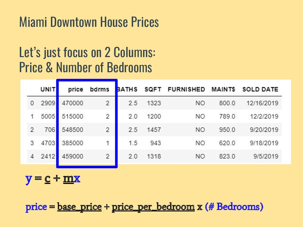
29. #Read data using Pandas df = pd.read_csv('../data/home_sales.csv') bdrms = df['bdrms'].values actual_prices = df['price'].values
30. with pm.Model() as home_price_model: #define priors base = pm.Uniform('base_price', 0, 500,000) ppb = pm.Uniform('price_per_bdrm', 0, 250,000) sigma = pm.HalfNormal('sigma', sd=100,000) y_predicted = base + ppb * bdrms #define Likelihood likelihood = pm.Normal('y', mu = y_predicted, sigma = sigma, observed = actual_prices)
31. with home_price_model: trace = pm.sample(2000, chains=2, tune=1000) The posterior is very hard to calculate analytically. So we resort to sampling from it a few 1000 times. (More on this later)
34. Examples of where Bayesian Analysis could be useful
35. 2 Hypothesis Problems • Does this person have the disease? • Will there be an earthquake (in the next t years)? • Actuary: Will there be flooding? • Will this person survive beyond 90 years of age? • Will it rain in September? (Agriculture) • Will they buy this product? (Y/N) once inside the store • Will the Cubs win next year? • Will we find oil in that exploration site? Lots and lots of Yes/No, Success/Failure outcomes
36. The Bayesian “Crank” Prior Probability New Evidence Posterior Probability Prior Probability New Evidence Posterior Probability Prior Probability New Evidence Posterior Probability
37. Before looking at the next example, let’s understand 2 distributions. These are closely related. Binomial Distribution Beta Distribution
38. Binomial Distribution
39. Intuition about the Binomial Distribution Let’s look at how things change: http://www.malinc.se/math/statistics/binomialen.php n = number of trials (samples) p = prob of getting a 1 (success) k or x = number of successes 0 or 1 outcomes 1 = “success” 0 = failure a binomial distribution (a series of successes and failures)
40. Image credit: https://math.stackexchange.com/questions/2123873/is-the-maximum-of-a-probability-distribution-function-of-a-binomial-distribution
41. Beta Distribution
42. Intuition about the Beta Distribution A whole class of distributions Two “free” parameters to describe it: alpha & beta The beta distribution is a continuous probability distribution that can be used to represent proportion or probability outcomes. For example, the beta distribution might be used to find how likely it is that your preferred candidate for mayor will receive 70% of the vote.
43. Beta Distributions Not only is the y-axis a probability (or more precisely a probability density), but the x-axis is as well. The Beta distribution is representing a probability distribution of probabilities.
44. Beta Distribution: A highly flexible distribution A very flexible distribution. Becomes the Uniform distribution if a=1, b=1 Beta → Normal if a=b for larger values of a and b
45. Intuition about and β is number of “successes” β often represents “misses” + β = Total attempts In Baseball: What could be and β? In Basketball: What could be and β? In Football (soccer): What could be and β? In marketing? In Oil Drilling? In Gambling? (Slot machines)
46. Updating Beta Distribution is VERY EASY With New evidence: Start with =1 and β=1 Take 1 new data point If you get a success, = +1 If you miss, β = β + 1 New Data Result β Starting 1 1 1 Success 1+1 1 2 Success 2+1 1 3 Fail 3 1+1 4 Success 3+1 2
47. Beta Distribution Binomial Distribution
48. How Beta and Binomial are related... IF you have a Binomial Likelihood, and a uniform prior… Then the posterior simplifies to a beta distribution! p( θ | y ) = beta(y+1, n-y+1) where y is number of successes out of n trials
49. How Beta and Binomial are related... IF you have a Binomial Likelihood, and a beta prior... Then the posterior is again a beta distribution! p( θ | y ) = beta(a+y, b+n-y) where y is number of successes out of n trials a and b are the prior shape parameters a ≈ “prior number of 1’s,” b ≈ “prior number of 0’s,” a+b ≈ “prior sample size.” n is our experiment sample size a+b is sometimes referred to as a running start
50. Conjugate Priors We say that the beta distribution is the conjugate prior for the binomial distribution, because when we combine the likelihood and prior, we get a posterior that has the form of the prior again: → another beta distribution. “Conjugate” here means that the posterior will follow the same distribution as the prior
51. Oil Exploration Example 2
52. Oil Exploration is expensive. Even after a Geological study, it is not certain that a given site will yield oil. In the last 2 years, a Nigerian Oil Investment company has sponsored 18 attempts. They’ve had 2 successes and 16 duds. Should they continue sponsoring? or Stop? Image: Market Business News Question: How certain can we be that there is at least a 10% chance of finding oil in any given prospective site?
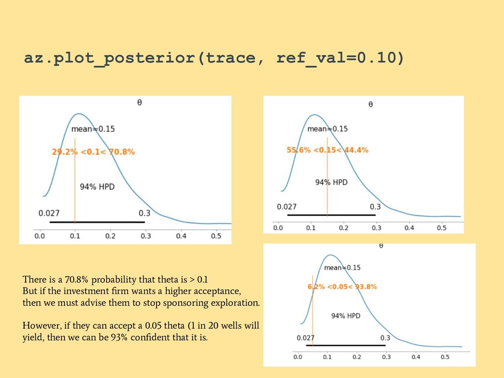
53. exploration_data = [0,0,0,1,0,0,0,0,0, 0,0,0,0,1,0,0,0,0] with pm.Model() as oil_exploration_model: θ = pm.Beta('θ', alpha=1., beta=1.) y = pm.Bernoulli('y', p=θ, observed=exploration_data) trace = pm.sample(1000, tune=3000) Notice that the entire pyMC3 model fits in 4-5 lines, including the data!
54. az.plot_trace(trace) az.summary_trace()
55. az.plot_posterior(trace)
56. az.plot_posterior(trace, ref_val=0.10) There is a 70.8% probability that theta is > 0.1 But if the investment firm wants a higher acceptance, then we must advise them to stop sponsoring exploration. However, if they can accept a 0.05 theta (1 in 20 wells will yield, then we can be 93% confident that it is.
57. MCMC
58. Inferencing (Sampling) The beauty of probabilistic programming is that you actually don't have to understand how the inference works in order to build models, but it certainly helps. Thomas Weicki
59. MCMC Sampling Monte Carlo: A simple simulation technique with a fancy name. Uses random numbers Markov Property says that given a process which is at a state Xn at a particular point of time, the probability of Xn+1=k, where k is another state the process can jump to, will only be dependent on its current state. And not on how it reached the current state.
60. Find the shape of the posterior, by sampling Intuitively, what we want to do is to walk around on some (lumpy) surface(our Markov chain) in such a way that the amount of time we spend in each location is proportional to the height of the surface at that location(our desired pdf from which we need to sample)
61. If we take the histograms of the draws, we get an estimate of the shape of the posterior distribution
62. A/B Testing Example 3
63. 900 100 59 liked 7 liked What can we conclude about Option 2 vs Option 1? Option 1 90% of the customers Option 2 10% of the customers
64. For a Bayesian Approach, we need Priors p1 ~ Uniform [0,1] p1 ~ beta (alpha=2, beta=2) p2 ~ beta (2, 2) Likelihood Binomial ~ N1, k1, p1 Binomial ~ N2, k2, p2 N customers, k “successes” p
65. Since we want to compare prior_opt1 with prior_opt2
68. ?
69. What next? Where to go from here?
71. Three Takeaways 1. If you look beyond the jargon, Bayesian Analysis is intuitive & easy to understand 2. The framework is robust. With modeling experience (and study) it is a nice addition to your toolkit 3. It is quite easy to get started on PyMC3 code
72. @ramnarasimhan
73. Resources: Coin Flipping Osvaldo Martin’s book (Bayesian Analysis with Python) gives a nice introductory overview to setting up variants of the Coin Tossing problem. (https://github.com/PacktPublishing/Bayesian-Analysis-with-Python-Second-Edition/blob/master/Chapter02/02%20Programming %20probabilistically.ipynb ) Here’s a blog post that summarizes it well: How to build probabilistic models with PyMC3 in Bayesian
74. Resources: Linear Regression Osvaldo Martin’s book (Bayesian Analysis with Python) gives a nice introductory overview to setting up variants of Linear Regression: https://github.com/PacktPublishing/Bayesian-Analysis-with-Python-Second-Edition/blob/master/Chapter03/03_Modeling%20with% 20Linear%20Regressions.ipynb
75. Resources: AB Testing with PyMC3 Will Kurt: An Introduction to Probability and Statistics | PyData New York 2019 https://github.com/willkurt/ProbAndStats-PyDataNYC2019/blob/master/noteboo ks/Part%203%20-%20Linear%20Models%20and%20PyMC3.ipynb Thiago Balbo's Blog post is simple and very accessible: Coding Bayesian AB Tests in Python to Optimize your App or Website Conversions example from Cam’s book: https://nbviewer.jupyter.org/github/CamDavidsonPilon/Probabilistic-Programmin g-and-Bayesian-Methods-for-Hackers/blob/master/Chapter2_MorePyMC/Ch2_ MorePyMC_PyMC3.ipynb
76. Resources Probabilistic Programming in Python using PyMC3: A very readable paper by the creators of PyMC3
77. PD vs PPD The posterior distribution refers to the distribution of the parameter whereas the predictive posterior distribution (PPD) refers to the distribution of future observations of data
78. Excellent Beginner’s Tutorial https://towardsdatascience.com/estimating-probabilities-with-bayesian-modeling-in-python-7144be007815
79. MCMC Details
80. Goal: To get hold of the Posterior Distribution The posterior distribution exists after the observed data has been incorporated into the model. However, due to the curse of dimensionality this posterior is inaccessible analytically. In order to approximate the posterior and do anything useful with your model, you must perform MCMC.
81. MCMC with the Math... • To begin, MCMC methods pick a random parameter value to consider. • The simulation will continue to generate random values (this is the Monte Carlo part), but subject to some rule for determining what makes a good parameter value. • The trick is that, for a pair of parameter values, it is possible to compute which is a better parameter value, by computing how likely each value is to explain the data, given our prior beliefs. • If a randomly generated parameter value is better than the last one, it is added to the chain of parameter values with a certain probability determined by how much better it is (this is the Markov chain part).
82. Intuition behind MCMC Algorithm 1. Start at a random initial State i. 2. Randomly pick a new Proposal State by looking at the transition probabilities in the ith row of the transition matrix P. 3. Compute a measure called the Acceptance Probability which is defined as: aij=min(sj.pji/si.pij,1). 4. Now Flip a coin that lands head with probability aij. If the coin comes up heads, accept the proposal, i.e. move to next state else reject the proposal, i.e. stay at the current state. 5. Repeat for a long time Core Intuition: If the spot probability (pdf) is high, sample from there more. This will contribute to an increased height of the histogram which we will plot. If the pdf at that spot is small, sample from there very little. Quickly, jump to some other spot in the probability space. https://towardsdatascience.com/mcmc-intuition-for-everyone-5ae79fff22b1
83. MC and MCMC MONTE CARLO • Use repeated random draws to approximate a target probability distribution. • Produce a sequence of draws that can be used to estimate unknown parameters. MARKOV CHAIN MONTE CARLO • Are a type of Monte Carlo sampler • Build a Markov Chain by starting at a specific state and making random changes to the state during each iteration • Result in a Markov Chain that converges to the target distribution Source: https://www.aptech.com/blog/fundamental-bayesian-samplers/
84. Inferencing (Sampling) MCMC generates samples from the posterior distribution https://twiecki.io/blog/2015/11/10/mcmc-sampling/ https://www.aptech.com/blog/fundamental-bayesian-samplers/
85. MCMC: Sampling the Posterior This is an area of active research to this day. As recently as in 2014, Andrew Gelman NUTS: No U-Turn Sampler is a form/variant of MCMC that is incredibly complex, but we can use it very easily. It has made computation significantly easier.
86. Parameter estimation One Parameter Models
87. One-Parameter Models a single unknown parameter Bayesian inference for two one-parameter models: 1. the binomial model 2. the Poisson model Use this to learn the basics of Bayesian data analysis: conjugate prior distributions predictive distributions confidence regions