Lab 1 - Introduction to Population Models in Excel and R

Transcript

1. Applied Population Dynamics Lab 1 – Excel and R Basics
2. Column B Referencing Equations Graphics R 2 / 24
3. Row 3 Referencing Equations Graphics R 3 / 24
4. Cell B3 Referencing Equations Graphics R 4 / 24
5. Create Sequence Using Auto-fill To use auto-fill: begin a sequence, highlight the cells, and then drag the box at the bottom-right of the last cell. Referencing Equations Graphics R 5 / 24
6. Relative Cell References Cell C2 will take on the value of A2 Referencing Equations Graphics R 6 / 24
7. Relative Cell References Cell C2 will take on the value of A2 Referencing Equations Graphics R 6 / 24
8. Relative Cell References Values of reference will change when using auto-fill Referencing Equations Graphics R 7 / 24
9. Absolute Cell References Dollar sign “locks” a reference so that auto-fill won’t change it Referencing Equations Graphics R 8 / 24
10. Absolute Cell References Dollar sign “locks” a reference so that auto-fill won’t change it Referencing Equations Graphics R 8 / 24
11. Partial Cell References Referencing Equations Graphics R 9 / 24
12. Equations Referencing Equations Graphics R 10 / 24
13. Equations Referencing Equations Graphics R 10 / 24
14. Equations Referencing Equations Graphics R 11 / 24
15. Equations Referencing Equations Graphics R 11 / 24
16. Formulas Referencing Equations Graphics R 12 / 24
17. Graphics Referencing Equations Graphics R 13 / 24
18. Graphics Add a line for males Referencing Equations Graphics R 14 / 24
19. Graphics Add a line for males Referencing Equations Graphics R 14 / 24
20. Customize Add legend Referencing Equations Graphics R 15 / 24
21. Customize Add axis labels Referencing Equations Graphics R 16 / 24
22. Customize Change line color Referencing Equations Graphics R 17 / 24
23. R – Software for statistical computing R can be downloaded here: https://www.r-project.org/ Referencing Equations Graphics R 18 / 24
24. R – Software for statistical computing R can be downloaded here: https://www.r-project.org/ You can use the graphical user interface that comes with R, or you can run R through a system like ESS+emacs (https://vgoulet.act.ulaval.ca/en/home/) or R Studio (https://www.rstudio.com/). Referencing Equations Graphics R 18 / 24
25. R – Software for statistical computing R can be downloaded here: https://www.r-project.org/ You can use the graphical user interface that comes with R, or you can run R through a system like ESS+emacs (https://vgoulet.act.ulaval.ca/en/home/) or R Studio (https://www.rstudio.com/). Most people use R Studio these days. Referencing Equations Graphics R 18 / 24
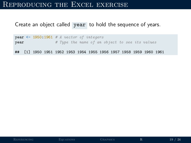
26. Reproducing the Excel exercise Create an object called year to hold the sequence of years. year <- 1950:1961 # A vector of integers year # Type the name of an object to see its values ## [1] 1950 1951 1952 1953 1954 1955 1956 1957 1958 1959 1960 1961 Referencing Equations Graphics R 19 / 24
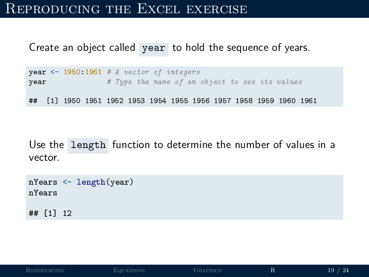
27. Reproducing the Excel exercise Create an object called year to hold the sequence of years. year <- 1950:1961 # A vector of integers year # Type the name of an object to see its values ## [1] 1950 1951 1952 1953 1954 1955 1956 1957 1958 1959 1960 1961 Use the length function to determine the number of values in a vector. nYears <- length(year) nYears ## [1] 12 Referencing Equations Graphics R 19 / 24
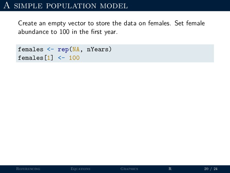
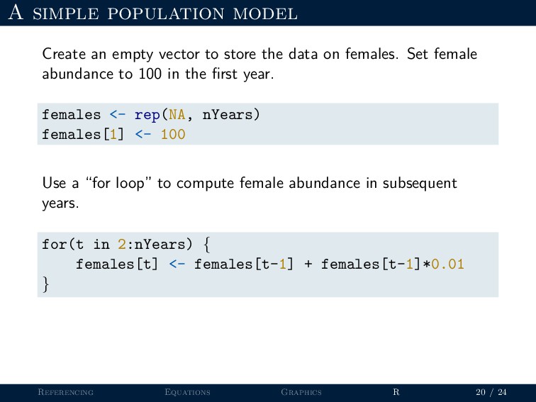
28. A simple population model Create an empty vector to store the data on females. Set female abundance to 100 in the first year. females <- rep(NA, nYears) females[1] <- 100 Referencing Equations Graphics R 20 / 24
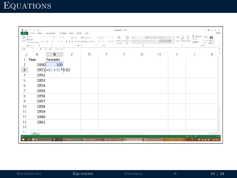
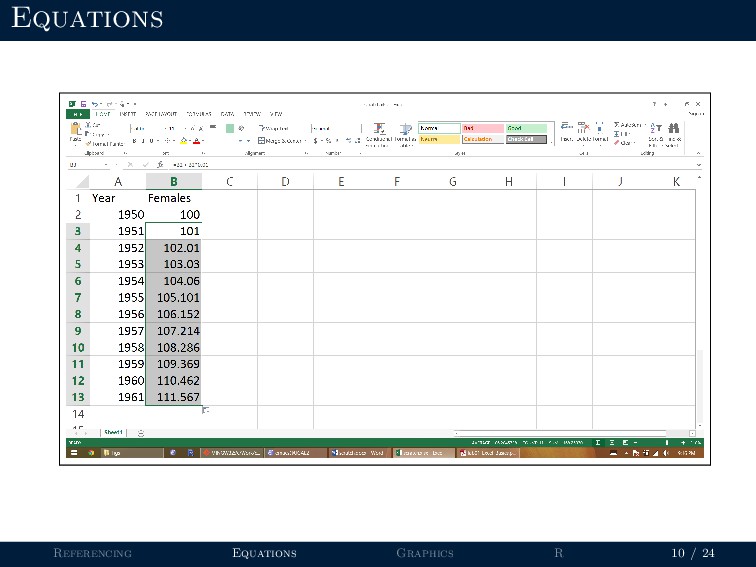
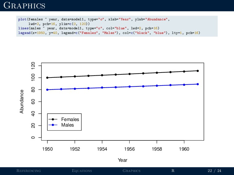
29. A simple population model Create an empty vector to store the data on females. Set female abundance to 100 in the first year. females <- rep(NA, nYears) females[1] <- 100 Use a “for loop” to compute female abundance in subsequent years. for(t in 2:nYears) { females[t] <- females[t-1] + females[t-1]*0.01 } Referencing Equations Graphics R 20 / 24
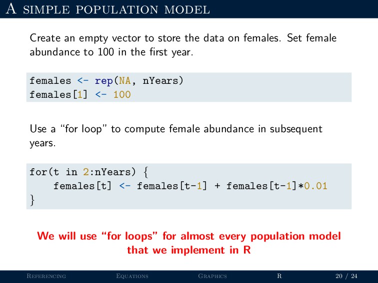
30. A simple population model Create an empty vector to store the data on females. Set female abundance to 100 in the first year. females <- rep(NA, nYears) females[1] <- 100 Use a “for loop” to compute female abundance in subsequent years. for(t in 2:nYears) { females[t] <- females[t-1] + females[t-1]*0.01 } We will use “for loops” for almost every population model that we implement in R Referencing Equations Graphics R 20 / 24
31. A simple population model Generate the data on males using a single line of code. males <- females*0.8 Referencing Equations Graphics R 21 / 24
32. A simple population model Generate the data on males using a single line of code. males <- females*0.8 Put the objects in a data.frame model1 <- data.frame(year, females, males) model1 ## year females males ## 1 1950 100.0000 80.00000 ## 2 1951 101.0000 80.80000 ## 3 1952 102.0100 81.60800 ## 4 1953 103.0301 82.42408 ## 5 1954 104.0604 83.24832 ## 6 1955 105.1010 84.08080 ## 7 1956 106.1520 84.92161 ## 8 1957 107.2135 85.77083 ## 9 1958 108.2857 86.62854 ## 10 1959 109.3685 87.49482 ## 11 1960 110.4622 88.36977 ## 12 1961 111.5668 89.25347 Referencing Equations Graphics R 21 / 24
33. Graphics plot(females ~ year, data=model1, type="o", xlab="Year", ylab="Abundance", lwd=2, pch=16, ylim=c(0, 120)) lines(males ~ year, data=model1, type="o", col="blue", lwd=2, pch=16) legend(x=1950, y=40, legend=c("Females", "Males"), col=c("black", "blue"), lty=1, pch=16) q q q q q q q q q q q q 1950 1952 1954 1956 1958 1960 0 20 40 60 80 100 120 Year Abundance q q q q q q q q q q q q q q Females Males Referencing Equations Graphics R 22 / 24
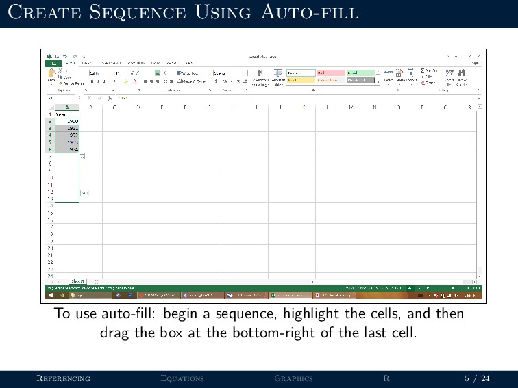
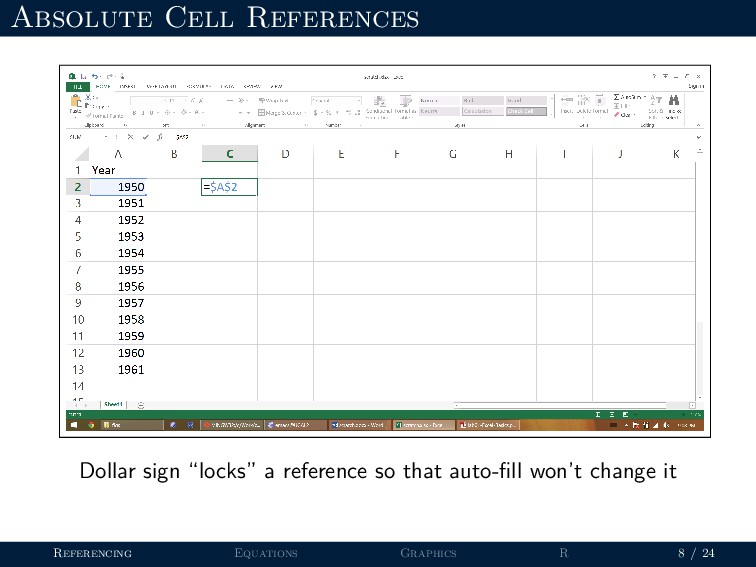
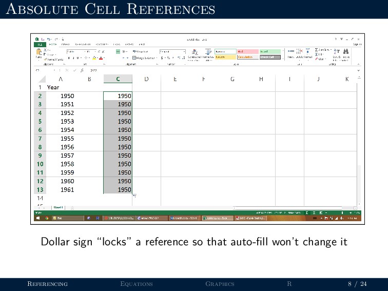
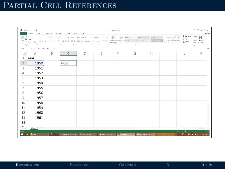
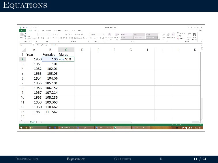
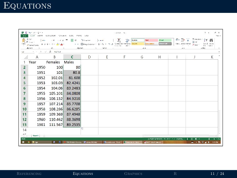
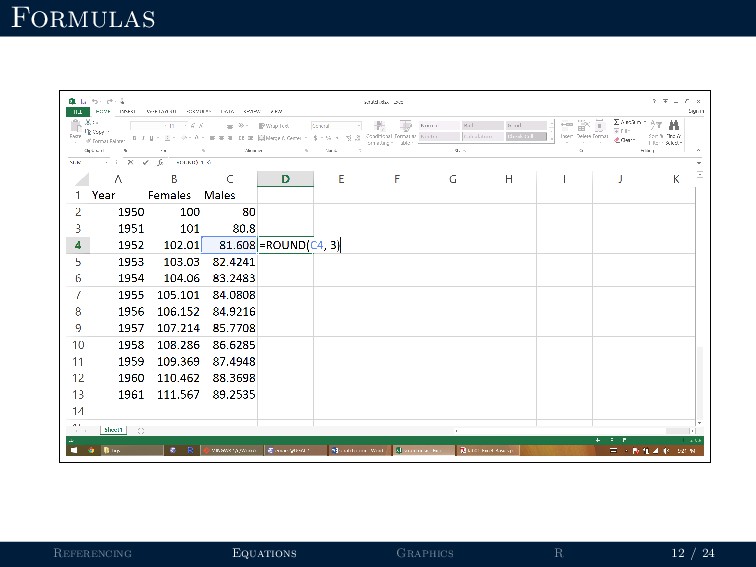
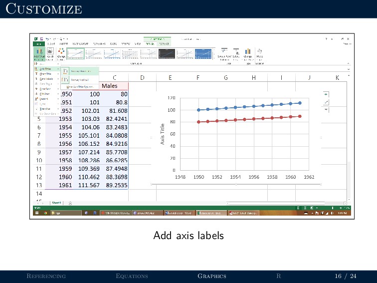
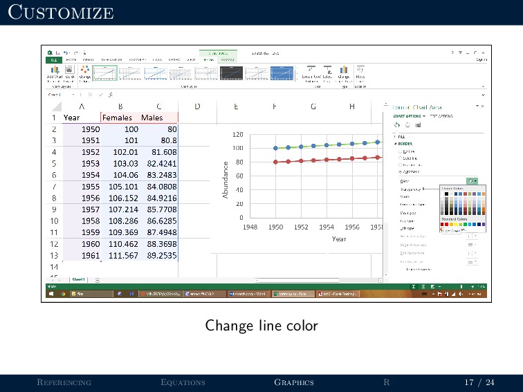
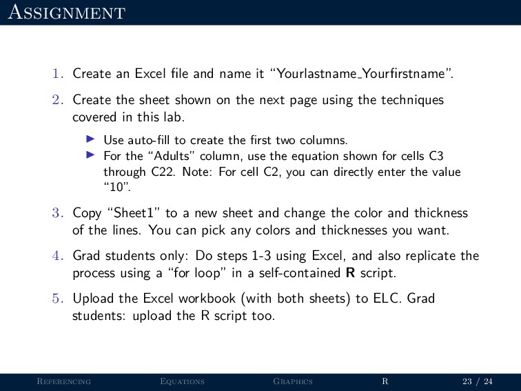
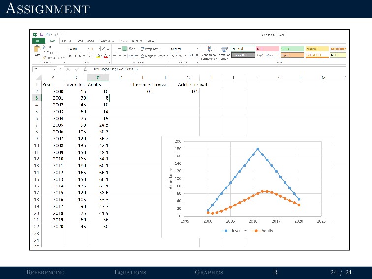
34. Assignment 1. Create an Excel file and name it “Yourlastname Yourfirstname”. 2. Create the sheet shown on the next page using the techniques covered in this lab. Use auto-fill to create the first two columns. For the “Adults” column, use the equation shown for cells C3 through C22. Note: For cell C2, you can directly enter the value “10”. 3. Copy “Sheet1” to a new sheet and change the color and thickness of the lines. You can pick any colors and thicknesses you want. 4. Grad students only: Do steps 1-3 using Excel, and also replicate the process using a “for loop” in a self-contained R script. 5. Upload the Excel workbook (with both sheets) to ELC. Grad students: upload the R script too. Referencing Equations Graphics R 23 / 24
35. Assignment Referencing Equations Graphics R 24 / 24