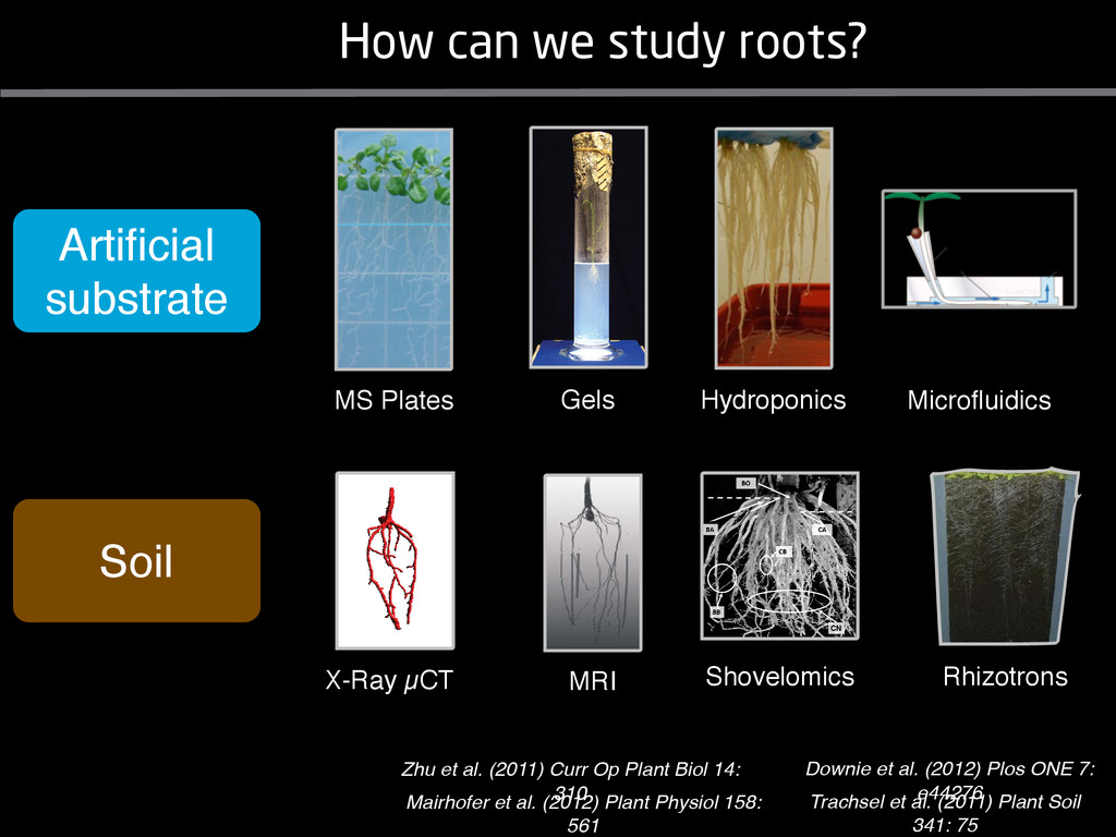
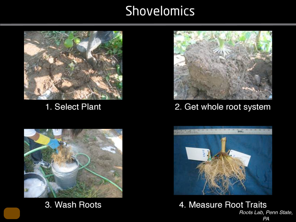
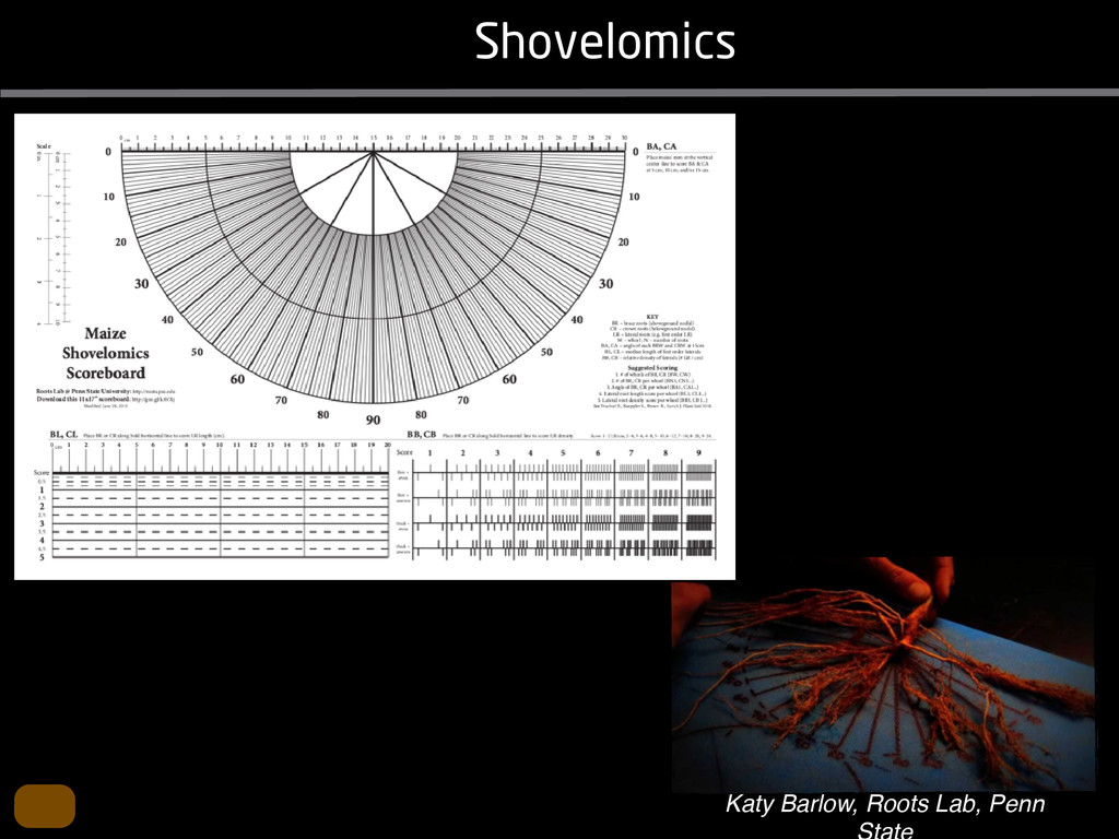
solidity, convex area, network area, and bushiness index. The definitions of each of these traits are as follows, where the abbreviation in parentheses denotes labels used in figures: (1) Median number of roots (MedR) is the result of a vertical line sweep in which the number of roots that crosses a horizontal line as the line moves vertically down the image was estimated, then the median of all values for the entire network was calculated. (2) Maximum number of roots (MaxR) is calculated by sorting the number of roots crossing a horizontal line in the vertical line sweep from smallest to largest, the max- imum number is considered to be the 84th percentile value (1 SD). MedR and MaxR computed using the line sweep approach give a good estimation when roots are well separated, but it can underestimate the number of roots when roots occlude each other. (3) Average root radius (Av. Radius) is the mean value of the root radius estimation computed for all pixels of the medial axis of the entire root system. (4) The total root length (Total Length) is the number of pixels in the medial axis of the root system. Note that estimating the length of the medial axis using Euclidean distance between pixels is a more rigorous calculation of the total root length, however our estimation computed as the number of Volume ¼ + N i¼1 pr2 i (6) SRL is the total root length divided by ro system volume. (7) Total surface area (SA) is estimate as a sum of circumferences of cross sections corr sponding to all pixels in the medial axis of the ro system: SA ¼ + N i¼1 2pri (8) Perimeter (Perim) is the total number of networ pixels connected to a background pixel (using 8-nearest neighbor neighborhood). (9) Convex are (ConvA) is the area of the convex hull that encom passes the image. Here, the convex hull is the smalle convex set of pixels that contains all other pixels in th root system. (10) Network area is the number network pixels in the root system. (11) Solidity is th fraction equal to the network area divided by th convex area. (12) Bushiness is the ratio of the max mum to the median number of roots. (13) Maximu width (Max Width) is a maximum horizontal width the whole RSA. (14) Depth is a maximum vertic distance reached by the root system. (15) Width-t Figure 1. Gel-based growth platform. A, 93-11 growing in gel in a 2 L ungraduated cylinder. The cylinder is placed on a lightbox on the imaging turntable and lit from the side. B, Images were acquired by zooming in on the root system. C, Cropped images from multiple angles were used for analysis. Approximately 20 angles (every 18°) from each plant were used for analysis; four are shown here. Iyer-Pascuzzi et al. MS Plates Gels Hydroponics Downie et al. (2012) Plos ONE 7: e44276 Microfluidics How can we study roots? Zhu et al. (2011) Curr Op Plant Biol 14: 310 Mairhofer et al. (2012) Plant Physiol 158: 561 Artificial substrate nique. RooTrak is able to visualize the contrasting fibrous and herring-bone root systems of monocot and dicot species, respectively. It is worth noting that the soils used in this study are typical United Kingdom field soils and not artificial media such as washed sands that have been used in many previous studies. Importantly we observed no difference in RooTrak root segmentation efficiency depending on soil type, which might have been expected since soil water content, a previously reported limitation of this tech- nique, is a function of soil texture. It should be noted that roots do not appear perfectly tubular all the time. This is due to the direction in which the cross section is taken and the complexity of branching structures, but also because of the nature of data representation. A voxel can sample two or more different components and as such the resulting intensity value is an average of all included values. The resolution at which data are captured or displayed also has a great influence, be it the two-dimensional image stack of mCT data or the 3D visualization of an object. Down-sampled data data can vary significantly between different visuali- zation techniques, introducing visual artifacts or leav- ing out important details, yet the 3D structure and complexity of the extracted root system architecture is still captured. It should be stressed that extraction of the descriptions shown in Figure 3 each required only a single mouse click from the user. To determine the success of RooTrak, its output should be compared to that obtained from other methods. Unfortunately, none of the previously reported software tools discussed here have been made publicly available. However, to form a point of comparison for the proposed tracking method, global thresholding was applied to each of the samples shown in Figure 3. Threshold boundaries were selected manually (compare with Lontoc-Roy et al., 2005, 2006), the operator trying to include as much root material as possible while at the same time reducing the amount of nonroot material extracted. Global thresholding is a very basic operation and therefore, in addition, a connectivity constraint based on a 26 neighborhood (compare with Lontoc- Roy et al., 2006; Perret et al., 2007) was applied. We believe that together these operations form a common denominator of previous root extraction methods from mCT data, though they do not correspond exactly to any given published technique. Root voxels were counted to compare the volumes extracted by both methods. The results are listed in Table II. Figure 4 provides a visual representation of a wheat plant root system extracted using global thresholding with connectivity checking and RooTrak, alongside an image of the root system obtained by washing the plant free from the surround- ing soil after the mCT scan. The result of global thresh- olding is typical: While the root architecture is present in the segmentation result, it is masked by a great many incorrectly labeled voxels. In Figure 4 these voxels may seem to be disconnected from the plant root system. Measured volume using global thresholding with a 26-neighbor connectivity constraint and RooTrak. The volume was calculated by counting the number of voxels and multiplying by the voxels’ size cubed. Plant Species Thresholding + Connectivity (Volume) RooTrak (Volume) mm3 Wheat 573.69 120.88 Wheat 558.75 76.94 Wheat 693.07 147.53 Maize 3,600.64 378.37 Tomato 270.24 22.58 Tomato 836.29 33.92 Figure 4. Results produced from the wheat scan by global thresholding with a 26-neighborhood connectivity constraint (A) and RooTrak (B). C, Image of washed root for comparison. 566 Plant Physiol. Vol. 158, 2012 X-Ray µCT can be performed in a much more direct and quantitative way than in humans. However, living plants do not have a ‘closed’ (hence com- pact) body layout, where internal surfaces separate organs which are connected by vessels. They rather show a so- called ‘open’ body plan, as they have to expose relatively large surfaces to the environment for maximal light intercep- tion, water and nutrient uptake. In order to fulfil this aim a branched structure is much more advantageous, but when considering them as MRI samples this leaves a lot of empty spaces between the ramified plant parts, resulting in a poor filling factor. Ideally, however, the r.f. and gradient coils should be very close to the interesting regions to achieve best noise figures and spatial resolution. Furthermore, plants have a ‘second half’ that is hidden in a completely different environment - the soil. MRI of roots can be even more challenging than that of the parts above ground, because delicate plant structures here are surrounded by water filled pores and often abundantly present para- or ferromagnetic impurities, which can result in image distor- tion. Even in terms of filling factors this scenario is typically worse than above ground, because healthy plants require big pots to grow. In those pots a lot of water is not associated with the plant, and this water has to be distinguished from signal arising form plant roots by suitable MRI contrast. Taken together the general shape of plants and its biodiversi- ty make MRI on living plants particularly demanding in terms of suitable hardware. Another factor that complicates matters is that plants have ‘aerenchyma’ leading to regions with small air pockets. Air conducts the magnetic field slightly different than water, which causes a local variation in the magnetic field. There- fore, an air bubble causes a magnetic field gradient, which will compete with the gradients used for the MRI experi- ment. The result is a loss of signal, mainly caused by diffu- sion in the local gradient and a dislocation of the water sig- nal in the image. In order to overcome some of the above problems, strong gradient coils are required in combination with high r.f. power, which is useful to shorten the echo times and therewith the time that diffusion can take place. This again is quite demanding on the equipment. A well equipped MRI lab for the investigation of plants therefore needs a variety of hardware solutions to match the various regions of interest. Additionally, a vertical bore magnet, high power gradient- and r.f.-coils are required, driven by strong amplifiers. Finally, for many plant experi- ments one should be able to control the environmental con- ditions inside the magnet with regard to light, temperature and humidity. 2.1 Contrast, spatial resolution and dynamic informa- tion A stated in section 1.2 MRI has a limited spatial resolution, which is often debated to be too low for microscopic appli- cations. For very small objects (diameter on the order of a or even sub-cellular level. However, this is an over- simplification. In many plant regions cell groups exist that exhibit roughly identical features, like overall size, relative compartment size, membrane permeability or sugar concen- tration. These cells can be taken together and viewed as an assembly. When special MRI sequences are then applied to such an assembly, averaged information can be acquired (like T2 , T1 , flow or translation diffusion, the four most commonly measured parameters). These MRI parameters can be translated on a pixel-by-pixel basis into morphologi- cal or physiological information which originates from the (sub-)cellular level, for instance: x vacuole size [5], x plasmalemma permeability [6], x relative sugar concentrations [7], x flow velocity, flow conducting area and volume flow in xylem and phloem [8,9] In a time series of experiments one can thus follow the dy- namical response of plant characteristics to varying envi- ronmental conditions by monitoring these or equally rele- vant, physiological parameters. Fig 2: 3D reconstruction of a maize root system in a 58 mm wide pipe. Three reference tubes were fixed to the outside allowing for concatenation of two 3D data sets. Field of view (FOV) is 68 × 68 × 130 mm, corresponding to 256 × 192 × 216 pixels. Time between excitation and echo detection, TE = 12 ms, recovery time between two succeeding experiments, TR = 3.5 s, slice thickness = 0.6 mm Albeit not a dynamical response of singular cells, the aver- aged response is often more than sufficient for plant physi- ology and biochemical studies. Such studies are therefore often restricted to two spatial coordinates, because generat- ing 3D maps of NMR parameters is time consuming and the focus of interest can typically be limited to one or a few slices through the plant. However, it is a nice feature of MRI that internal and external features of the sample can easily be recorded in 3D. If we limit ourselves to obtaining an appro- priate contrast between tissues, as is common for MRI stu- dies in the medical field, the duration of such 3D measure- ments does not become too excessive (e.g. 30 min) and can be used to study the development of morphological features. Figure 2 shows an example of a maize plant with its roots in normal sand that is not fully saturated with water. The roots sit in a plastic pipe with 3 reference tubes attached to it to allow for concatenation. This image shows a MRI was carried out without plants for 10 days. Ca(NO3 )2 , 0.25 mM KH2 PO Figure 1. The rhizotron system called ‘‘Ara-rhizotron’’ for growing Arabidopsis plants in population. the Ara-rhizotron including four pieces of PVC (one back sheet and three borders) and the front sh Ara-rhizotron is 49 cm high, 24 cm wide, and 1.3 cm thick with tongs for a usable space of 47 c 3 mm thick. The irrigation system consists of three connectors independent placed at the back of th away of the Ara-rhizotron box showing the disposition of the seven Ara-rhizotrons in each box, wit tion to the vertical and separated from each other by 4 cm. The polycarbonate transparent sheets w the Ara-rhizotrons. (c) 33-day-old Arabidopsis plants grown in an Ara-rhizotron. Rhizotrons where one indicates shallow root angles (10°), low root numbers and a low branching density (0.5 lateral root cm−1). Nine indicates steep root angles (90°), high numbers and a high branching density (7 lateral roots cm−1). Representative images depicting con- trasts for the various traits are given in Fig. 2. Scoring in 2008 was carried out by a different researcher than in 2009 and 2010. Correlations between traits were established using the Spearman- Rank correlation. Significant correlations between traits with r<0.5 were considered weak, 0.5<r<0.8 moderate and r>0.8 strong. four times. In 2009, excavated root crowns were visually scored and subsequently used to measure root angles and to count numbers of brace roots, crown roots and lateral roots originating from brace and crown roots. Angles of roots were measured using a large protractor. The number of lateral roots was counted on a 4 cm root segment obtained from 5 cm below the soil surface. On the same 4 cm segment the mean length of 3 randomly selected lateral roots was measured. Linear density was calculated as the number of lateral roots per cm. Root angles for crown and brace roots were averaged after measuring the angles of three typical roots for each root class. In 2010 30 IBM RILs were randomly selected to evaluate how the accuracy of scoring for CN and CA would be affected by removing the brace roots on one side of the root crown. Prior to scoring of CN and CA brace roots were removed from one side of the root crown. CN and CA were thereafter scored as described above. Subsequently CN were counted and CA measured with a large protractor. Trait values obtained by scoring and counting (CN)/measuring (CA) were thereafter correlated. Significant correlations be- tween traits with r<0.5 were considered weak, 0.5< r<0.8 moderate and r>0.8 strong. Variability among plants was assessed by comparing the values measured on the three root crowns excavated for one genotype. Variability is described using the coefficient of variation (C.V.). Results Large variability was observed among genotypes Phenotypes varied widely in both years and environ- ments within and between populations (Figs. 2 and 3). Scores for the number of brace roots (BO), the angles (BA) and branching (BB) of brace roots ranged from Fig. 1 Ten traits were assessed visually on the excavated root crowns: number of whorls occupied by brace roots (BW), number of brace roots (BO), 1st (BA1a, BA2a) and 2nd (BA1b, BA2b) arm of the brace roots originating from whorl 1, whorl 2, respectively, the branching density of brace roots (BB), the number (CN), angles (CA) and branching density (CB) of crown roots Plant Soil (2011) 341:75–87 79 Shovelomics Soil Trachsel et al. (2011) Plant Soil 341: 75