Learning Deep neural network (DNN) surrogate models for UQ

Presentation at SIAM UQ 2018.

Transcript

1. Learning Deep neural network (DNN) surrogate models for UQ Rohit Tripathy, Ilias Bilionis Predictive Science Lab School of Mechanical Engineering Purdue University Arxiv: https://arxiv.org/abs/1802.00850
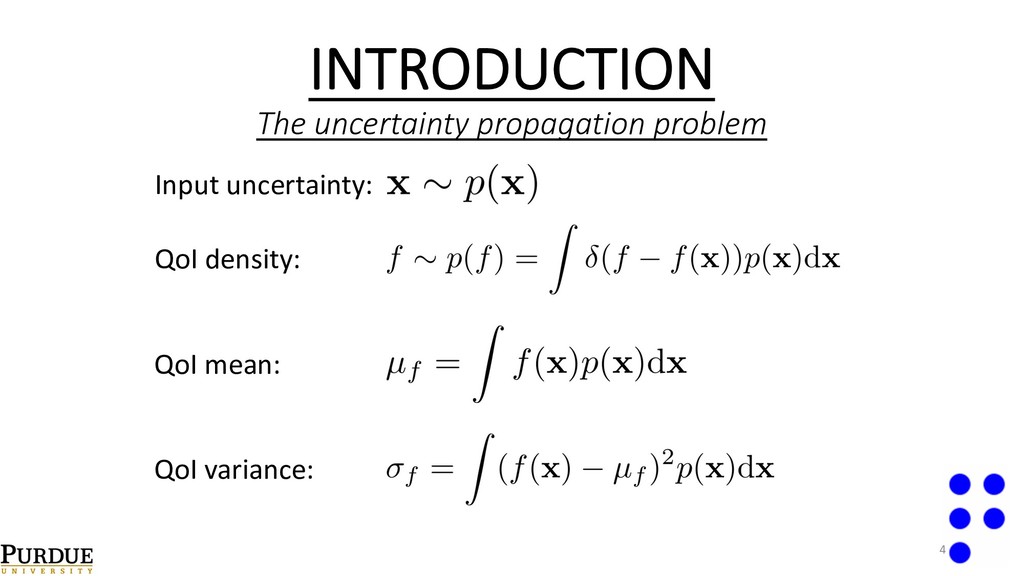
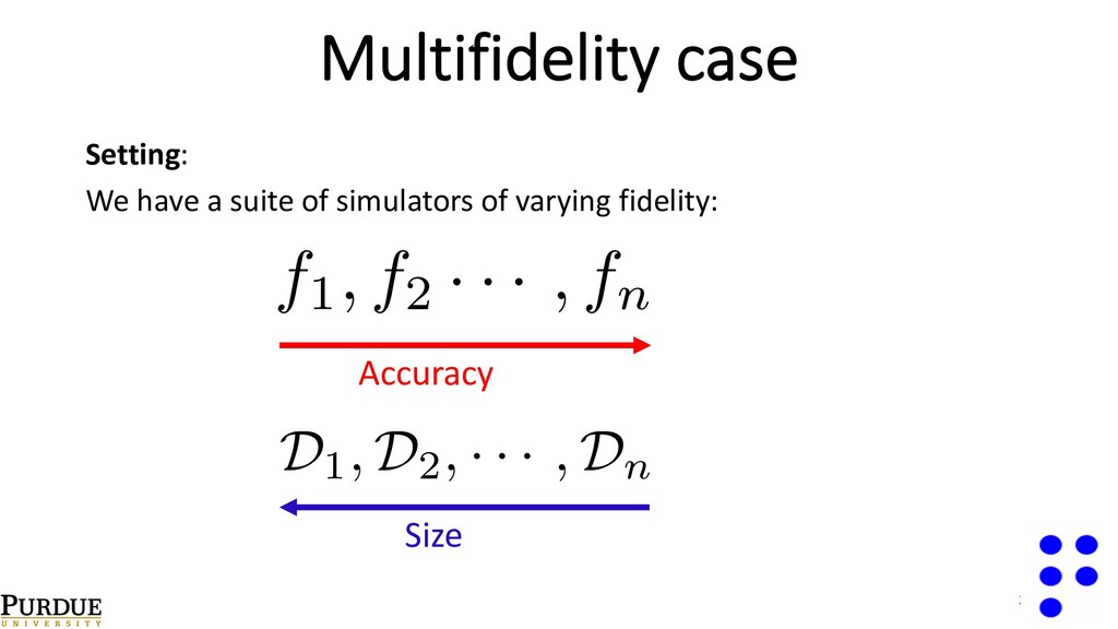
2. INTRODUCTION Image sources: [1] - Left image. [2] - Right image.. - f is some scalar quantity of interest. - Obtained numerically through the solution of a set of PDEs. - Inputs x – uncertain and high dimensional. - Interested in quantifying the uncertainty in f. 3
3. INTRODUCTION The uncertainty propagation problem Input uncertainty: QoI density: QoI mean: QoI variance: 4
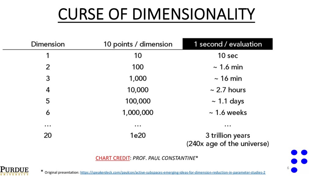
4. • The expectations have to be computed numerically. • Monte Carlo, although independent in the dimensionality, converges very slowly in the number of samples of f. • Idea -> Replace the simulator of f with a surrogate model. • Problem -> Curse of dimensionality. 5
5. CURSE OF DIMENSIONALITY CHART CREDIT: PROF. PAUL CONSTANTINE* * Original presentation: https://speakerdeck.com/paulcon/active-subspaces-emerging-ideas-for-dimension-reduction-in-parameter-studies-2 6
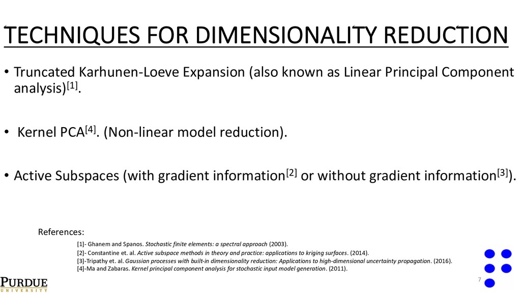
6. TECHNIQUES FOR DIMENSIONALITY REDUCTION • Truncated Karhunen-Loeve Expansion (also known as Linear Principal Component analysis)[1]. • Kernel PCA[4]. (Non-linear model reduction). • Active Subspaces (with gradient information[2] or without gradient information[3]). References: [1]- Ghanem and Spanos. Stochastic finite elements: a spectral approach (2003). [2]- Constantine et. al. Active subspace methods in theory and practice: applications to kriging surfaces. (2014). [3]-Tripathy et. al. Gaussian processes with built-in dimensionality reduction: Applications to high-dimensional uncertainty propagation. (2016). [4]-Ma and Zabaras. Kernel principal component analysis for stochastic input model generation. (2011). 7
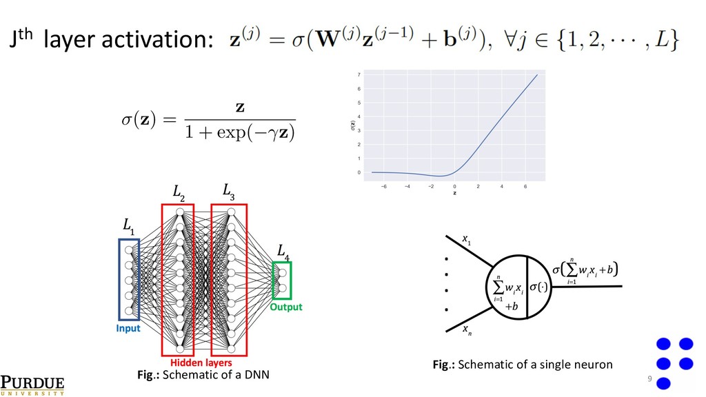
7. DEEP NEURAL NETWORKS o Universal function approximators[1]. o Layered representation of information[2]. o Linear regression can be thought of as a special case of DNNs (no hidden layers). o Tremendous success in recent times in applications such as image classification[2], autonomous driving[3]. o Availability of libraries such as tensorflow, keras, theano, PyTorch, caffe etc. References: [1]-Hornik . Approximation capabilities of multilayer feedforward networks. (1991). [2]-Krishevsky et al. Imagenet classification with deep convolutional neural networks. (2012). [3]-Chen et. al. Deepdriving: Learning affordance for direct perception in autonomous driving. (2015). 8
8. Fig.: Schematic of a DNN Fig.: Schematic of a single neuron 9 Jth layer activation: (z) = z 1 + exp( z)
9. NETWORK ARCHITECTURE f(x) = h(g(x)) Surrogate Link Projection D Active subspace: 10
10. 11 TRAINING A DNN Discrepancy / log likelihood Regularizer / Log prior ✓ = {Wi, bi }L i=1 All network parameters (weights and biases): Loss function: SGD update:
11. Model selection BGO 12
12. Stochastic Elliptic Partial Differential Equation r(a(x)ru(x)) = 0, x = (x1, x2) 2 ⌦ = [0, 1]2, u = 0, 8x1 = 1, u = 1, 8x1 = 0, @u @n = 0, 8x2 = 1. PDE: Boundary conditions: Uncertain diffusion: Exponential covariance: 13 log
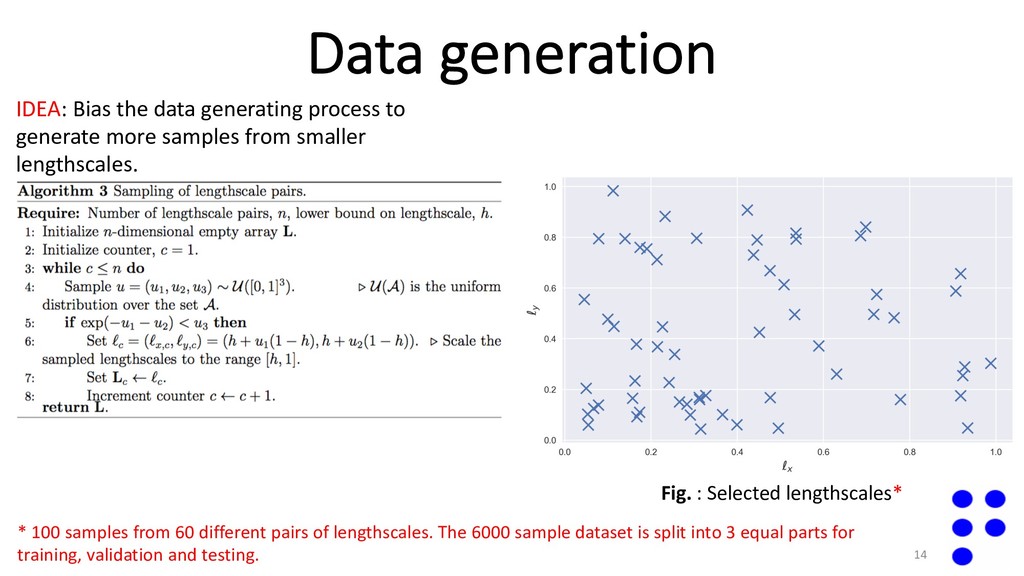
13. Data generation IDEA: Bias the data generating process to generate more samples from smaller lengthscales. 14 Fig. : Selected lengthscales* * 100 samples from 60 different pairs of lengthscales. The 6000 sample dataset is split into 3 equal parts for training, validation and testing.
14. Results 15 1. Model selection results Fig. : BGO for selecting regularization constant corresponding to L = 7, d = 2. Fig. : Heatmap of validation error over grid of L and h. Lowest Validation error
15. 16 2. Test set predictions
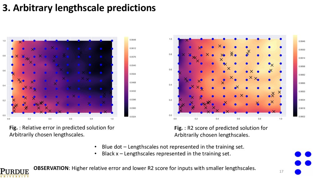
16. 17 3. Arbitrary lengthscale predictions Fig. : Relative error in predicted solution for Arbitrarily chosen lengthscales. Fig. : R2 score of predicted solution for Arbitrarily chosen lengthscales. • Blue dot – Lengthscales not represented in the training set. • Black x – Lengthscales represented in the training set. OBSERVATION: Higher relative error and lower R2 score for inputs with smaller lengthscales.
17. Uncertainty propagation example 18 Fig. : Comparison of Monte Carlo* (left) mean and variance and surrogate (right) mean and variance for the PDE solution. Lengthscales: * 106 MC samples.
18. 19 Fig.: Comparison of solution pdf at x = (0.484,0.484) obtained from MCS* and DNN surrogate. Fig.: Comparison of solution pdf at x = (0.328, 0.641) obtained from MCS* and DNN surrogate. * 106 MC samples.
19. Setting: We have a suite of simulators of varying fidelity: 20 Multifidelity case f1, f2 · · · , fn Accuracy D1, D2, · · · , Dn Size
20. 21 Multi-output network structure y1 y2 yn OUTPUTS h g D = {D1, D2, · · · , Dn } Denote all datasets collectively as: Loss function: L(✓, DM ) = n X i=1 Li(✓, DM ) + R(✓) Lt(✓, Xj, yi,j) = I t(i) ⇥ L(✓, Xj, yi,j) t, fidelity index
21. 22 Elliptic PDE revisited r(a(x)ru(x)) = 0, x = (x1, x2) 2 ⌦ = [0, 1]2, u = 0, 8x1 = 1, u = 1, 8x1 = 0, @u @n = 0, 8x2 = 1. PDE: Boundary conditions: Uncertain diffusion: Exponential covariance:
22. 23 `x = 0.3, `y = 0.3 Lengthscales: KL expansion: log a(x) = N X i=1 p i i(x)⇠i. N = 350 # terms: Elliptic PDE revisited Bi-fidelity dataset size: Nlow = 900, Nhigh = 300
23. 24 Fig. : How many samples of the purely high fidelity dataset would we need to converge to the reduce the error obtained through the multifidelity case ?
24. FUTURE WORK • Explore better ways of parameterizing the network. • Explore Bayesian surrogates. • Fully convolutional architectures – arbitrarily shaped inputs. THANK YOU ! 25 Slides: https://speakerdeck.com/rohitkt10/dnn-for-hd-uq