Learning MsFEM basis functions using DNNs

Talk given at SIAM CSE 2017 conference on using deep neural networks for learning surrogate models for stochastic MsFEM basis functions.

Transcript

1. Learning Multiscale Stochastic Finite Element Basis Functions with Deep Neural Networks Rohit Tripathy and Ilias Bilionis Predictive Science Lab http://www.predictivesciencelab.org/ Purdue University West Lafayette, IN, USA
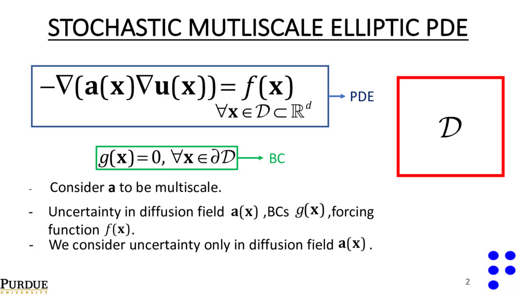
2. STOCHASTIC MUTLISCALE ELLIPTIC PDE D ∀x ∈D ⊂ !d 2 −∇(a(x)∇u(x))= f (x) g(x)= 0, ∀x ∈∂D PDE BC a(x) - Uncertainty in diffusion field ,BCs ,forcing function . a(x) f (x) g(x) - We consider uncertainty only in diffusion field . - Consider a to be multiscale.
3. MULTISCALE FEM (MsFEM)[1] 3 D K K i Solve: −∇(a(x)∇u(x))= 0∀x ∈K i u(x)= u j ∀x ∈∂K i KEY STEP ! Couple adaptive basis functions with full FEM solver. Reference: [1]-Efendiev and Hou, Multiscale finite element methods: theory and applications. (2009)
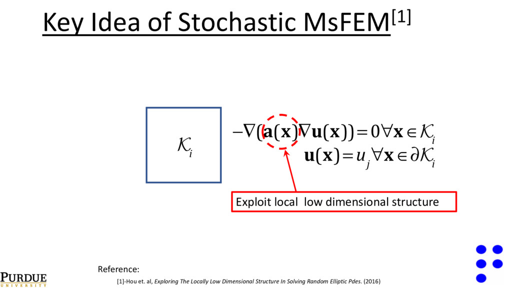
4. 4 K i −∇(a(x)∇u(x))= 0∀x ∈K i u(x)= u j ∀x ∈∂K i Key Idea of Stochastic MsFEM[1] Exploit local low dimensional structure Reference: [1]-Hou et. al, Exploring The Locally Low Dimensional Structure In Solving Random Elliptic Pdes. (2016)
5. Curse of dimensionality 5 CHART CREDIT: PROF. PAUL CONSTANTINE* * Original presentation: https://speakerdeck.com/paulcon/active-subspaces-emerging-ideas-for-dimension-reduction-in-parameter-studies-2
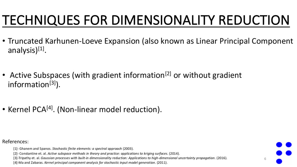
6. TECHNIQUES FOR DIMENSIONALITY REDUCTION • Truncated Karhunen-Loeve Expansion (also known as Linear Principal Component analysis)[1]. • Active Subspaces (with gradient information[2] or without gradient information[3]). • Kernel PCA[4]. (Non-linear model reduction). 6 References: [1]- Ghanem and Spanos. Stochastic finite elements: a spectral approach (2003). [2]- Constantine et. al. Active subspace methods in theory and practice: applications to kriging surfaces. (2014). [3]-Tripathy et. al. Gaussian processes with built-in dimensionality reduction: Applications to high-dimensional uncertainty propagation. (2016). [4]-Ma and Zabaras. Kernel principal component analysis for stochastic input model generation. (2011).
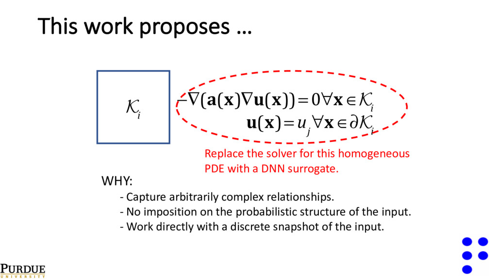
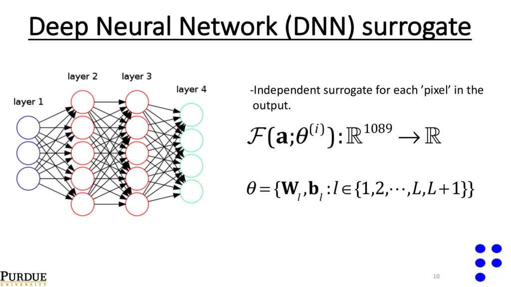
7. This work proposes … 7 K i −∇(a(x)∇u(x))= 0∀x ∈K i u(x)= u j ∀x ∈∂K i Replace the solver for this homogeneous PDE with a DNN surrogate. WHY: - Capture arbitrarily complex relationships. - No imposition on the probabilistic structure of the input. - Work directly with a discrete snapshot of the input.
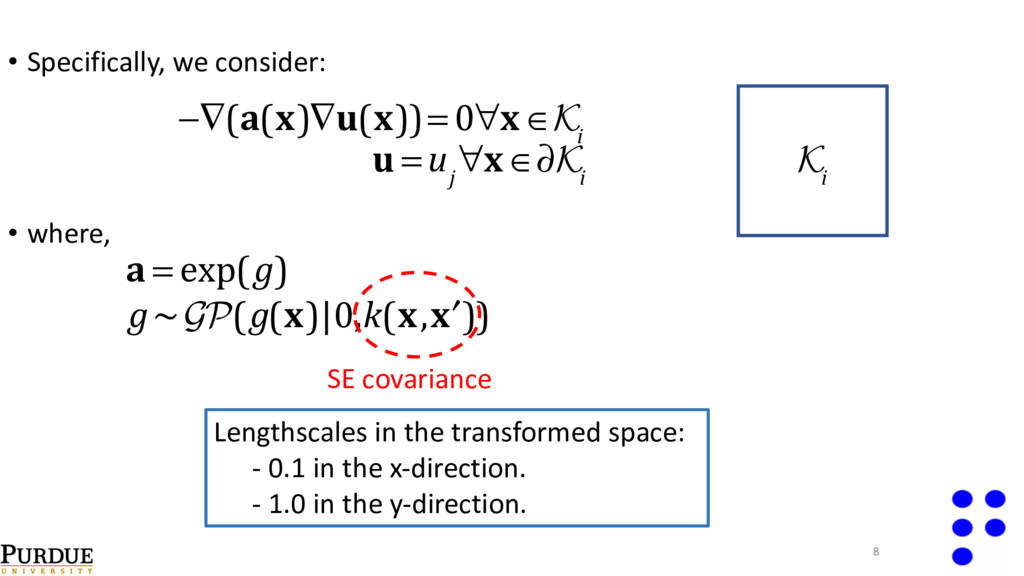
8. • Specifically, we consider: • where, g~GP(g(x)|0,k(x, ′ x )) 8 −∇(a(x)∇u(x))= 0∀x ∈K i K i a = exp(g) u = u j ∀x ∈∂K i SE covariance Lengthscales in the transformed space: - 0.1 in the x-direction. - 1.0 in the y-direction.
9. 9 SOLVER
10. Deep Neural Network (DNN) surrogate 10 -Independent surrogate for each ’pixel’ in the output. F(a;θ(i)):!1089 → ! θ = {W l ,b l :l ∈{1,2,!,L,L+1}}
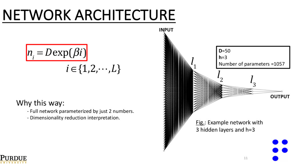
11. NETWORK ARCHITECTURE INPUT OUTPUT l 1 l 2 Fig.: Example network with 3 hidden layers and h=3 11 n i = Dexp(βi) i ∈{1,2,!,L} l 3 D=50 h=3 Number of parameters =1057 Why this way: - Full network parameterized by just 2 numbers. - Dimensionality reduction interpretation.
12. OPTIMIZATION Likelihood model: Full Loss function: NEGATIVE LOG LIKELIHOOD REGULARIZER 12 L j (θ,λ,σ ;a j )= log(σ )+ 1 2σ 2 ( y j − F(a j ;θ))2 y|a,θ,σ ~ N (|F(a,θ),σ 2) θ* ,σ * ,λ* = argminL L = 1 N j=1 N ∑L j + λ l=1 L+1 ∑oW l o 2
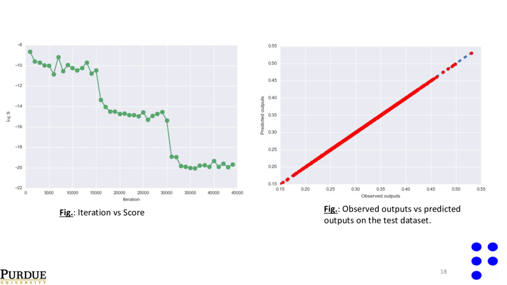
13. o Backpropagation[2] to compute gradients. o Use mini-batch size of 32. o Initial stepsize set to 3x10-4 . o Drop stepsize by factor of 1/10 every 15k iterations. o Train for 45k iterations. o Moment decay rate: . β 1 = 0.9,β 2 = 0.999 θ t =θ t−1 −α m t v t +ε 13 ADAptive Moments (ADAM[1]) optimizer References: [1]- Kingma and Ba. Adam: A method for stochastic optimization. (2014). [2]- Rummelhart and Yves, Backpropagation: theory, architectures, and applications. (1995).
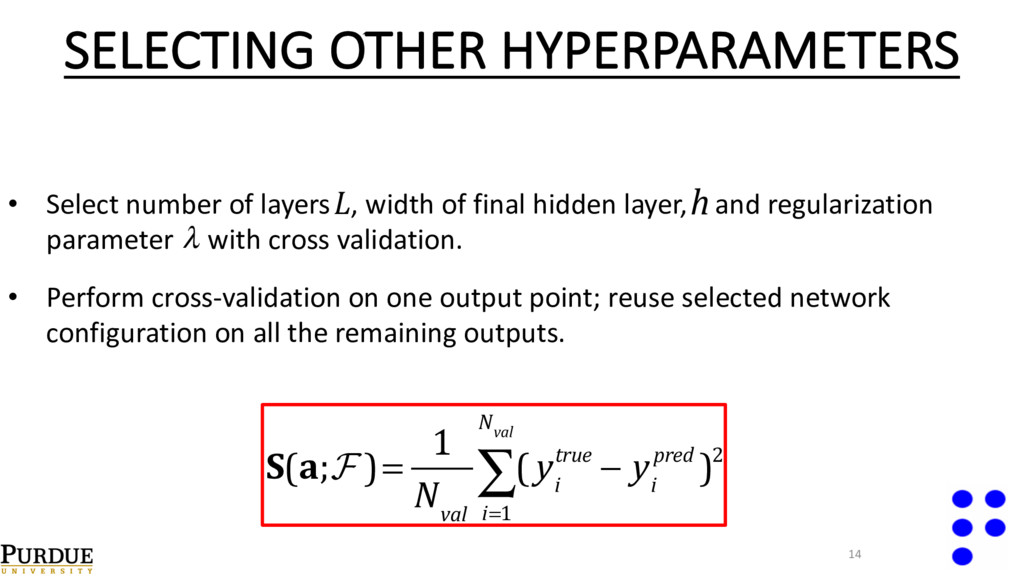
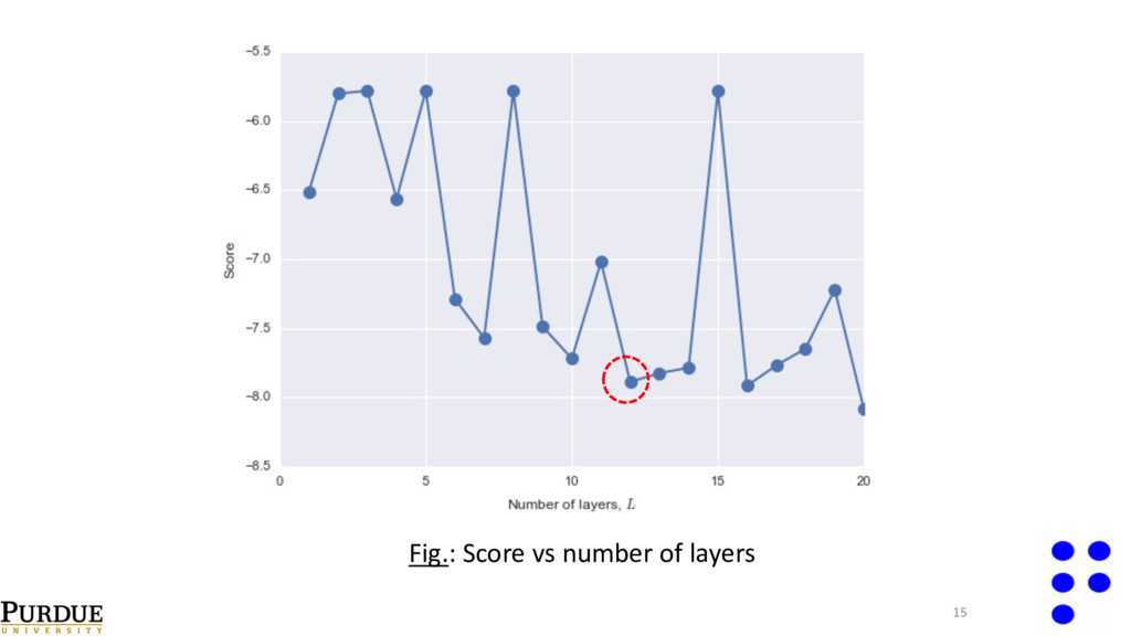
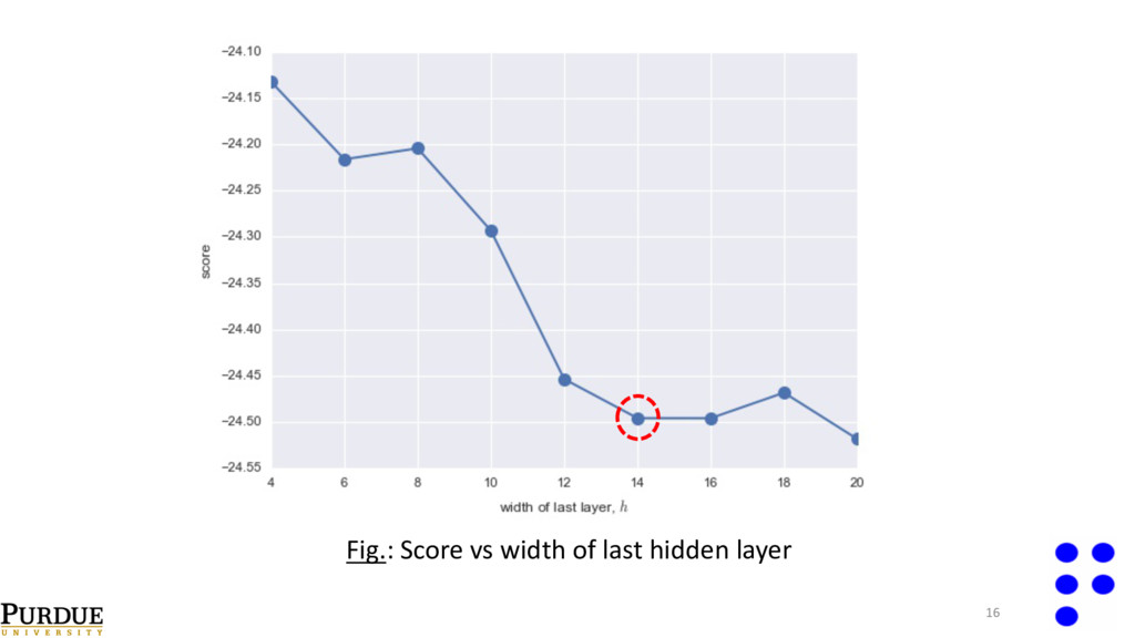
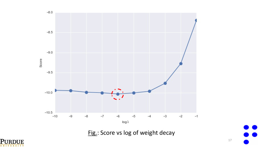
14. SELECTING OTHER HYPERPARAMETERS L h 14 S(a;F )= 1 N val i=1 N val ∑( y i true − y i pred )2 • Select number of layers , width of final hidden layer, and regularization parameter with cross validation. • Perform cross-validation on one output point; reuse selected network configuration on all the remaining outputs. λ
15. Fig.: Score vs number of layers 15
16. Fig.: Score vs width of last hidden layer 16
17. Fig.: Score vs log of weight decay 17
18. Fig.: Iteration vs Score Fig.: Observed outputs vs predicted outputs on the test dataset. 18
19. Prediction of full solution 19 MSE (x10-6): Predicted solution True solution
20. What if we predict solution on inputs from random fields that have different lengthscales ? 20
21. TESTING THE SURROGATE WITH DIFFERENT RANDOM FIELDS 21
22. 22 What about fields with discontinuities?
23. 23 PREDICTED SOLUTION TRUE SOLUTION
24. FUTURE DIRECTIONS • Reduce data with unsupervised pretraining. • Correlations between outputs (Multi-task learning). • Fields with arbitrary spatial discretization (Fully convolutional networks). • Bayesian training (stochastic variational inference). 24