Discovering nonlinear active subspace with DNNs

Poster presented at SIAM DR 2017 workshop.

Transcript

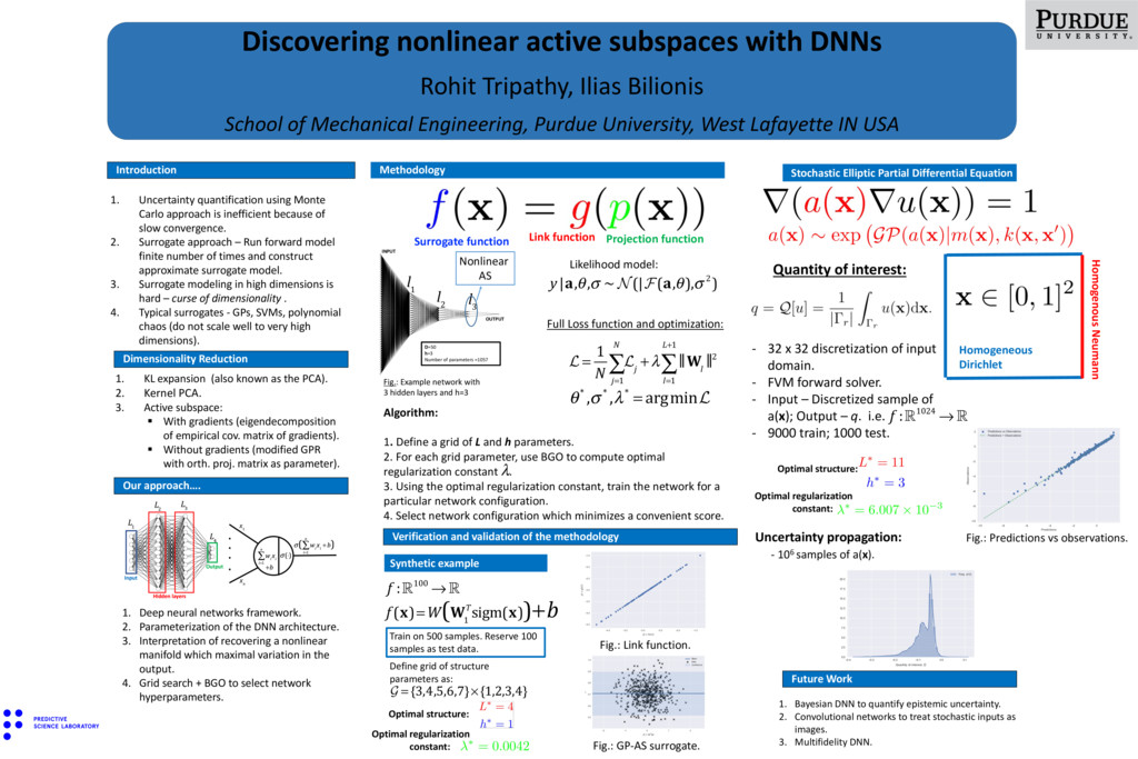
1. Discovering nonlinear active subspaces with DNNs Rohit Tripathy, Ilias Bilionis School of Mechanical Engineering, Purdue University, West Lafayette IN USA 1. Uncertainty quantification using Monte Carlo approach is inefficient because of slow convergence. 2. Surrogate approach – Run forward model finite number of times and construct approximate surrogate model. 3. Surrogate modeling in high dimensions is hard – curse of dimensionality . 4. Typical surrogates - GPs, SVMs, polynomial chaos (do not scale well to very high dimensions). Methodology Our approach…. 1. Deep neural networks framework. 2. Parameterization of the DNN architecture. 3. Interpretation of recovering a nonlinear manifold which maximal variation in the output. 4. Grid search + BGO to select network hyperparameters. Introduction Future Work Verification and validation of the methodology Synthetic example Stochastic Elliptic Partial Differential Equation 1. Bayesian DNN to quantify epistemic uncertainty. 2. Convolutional networks to treat stochastic inputs as images. 3. Multifidelity DNN. Dimensionality Reduction 1. KL expansion (also known as the PCA). 2. Kernel PCA. 3. Active subspace: § With gradients (eigendecomposition of empirical cov. matrix of gradients). § Without gradients (modified GPR with orth. proj. matrix as parameter). D=50 h=3 Number of parameters =1057 Fig.: Example network with 3 hidden layers and h=3 l 1 l 2 l 3 INPUT OUTPUT f (x)=W(W 1 Tsigm(x))+b Surrogate function Projection function Link function y|a,θ,σ ~ N (|F(a,θ),σ 2) Likelihood model: L = 1 N j=1 N ∑L j + λ l=1 L+1 ∑oW l o 2 Full Loss function and optimization: θ* ,σ * ,λ* = argminL Algorithm: 1. Define a grid of L and h parameters. 2. For each grid parameter, use BGO to compute optimal regularization constant . 3. Using the optimal regularization constant, train the network for a particular network configuration. 4. Select network configuration which minimizes a convenient score. λ f :!100 → ! Train on 500 samples. Reserve 100 samples as test data. Fig.: Link function. Define grid of structure parameters as: G = {3,4,5,6,7}×{1,2,3,4} Optimal structure: Optimal regularization constant: Fig.: GP-AS surrogate. Homogeneous Dirichlet Homogenous Neumann Quantity of interest: - 32 x 32 discretization of input domain. - FVM forward solver. - Input – Discretized sample of a(x); Output – q. i.e. - 9000 train; 1000 test. f :!1024 → ! Optimal structure: Optimal regularization constant: Uncertainty propagation: - 106 samples of a(x). Fig.: Predictions vs observations. Nonlinear AS